by Dan Rutherford
1. Legendrian and transverse knots
The basic objects of study are as follows: A contact structure on a 3-manifold is a maximally nonintegrable 2-plane field. A Legendrian (resp. transverse) knot in a contact 3-manifold, \( (M, \xi) \), is a smoothly embedded closed curve in \( M \) that is everywhere tangent (resp. everywhere transverse) to \( \xi \). Legendrian and transverse knots play a key role in 3- and 4-dimensional contact and symplectic topology similar to that of knots and links in low-dimensional topology, e.g., allowing for construction of manifolds via surgery/handle attachment or branched covering. Moreover, as indicated by Bennequin’s work (see Section 2.2 below) and the tight/overtwisted dichotomy subsequently discovered by Eliashberg, the behavior of Legendrian knots can reflect properties of the contact manifolds that they populate.
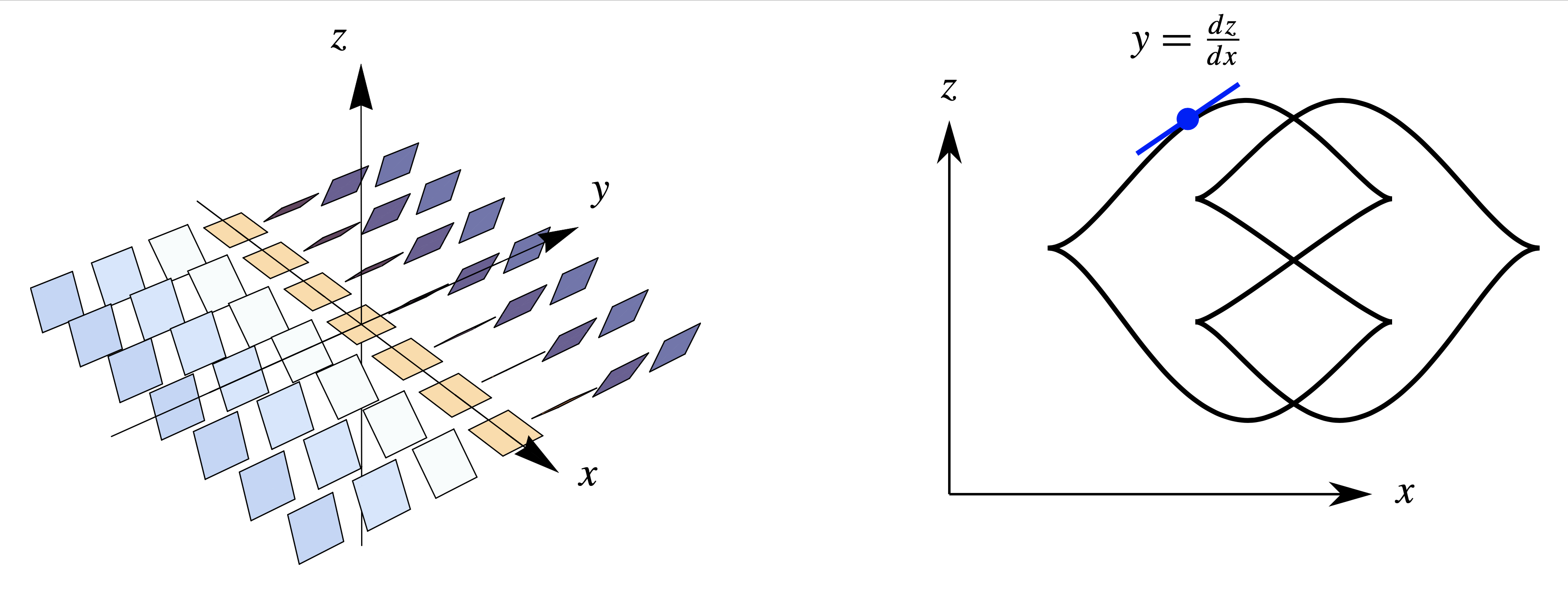
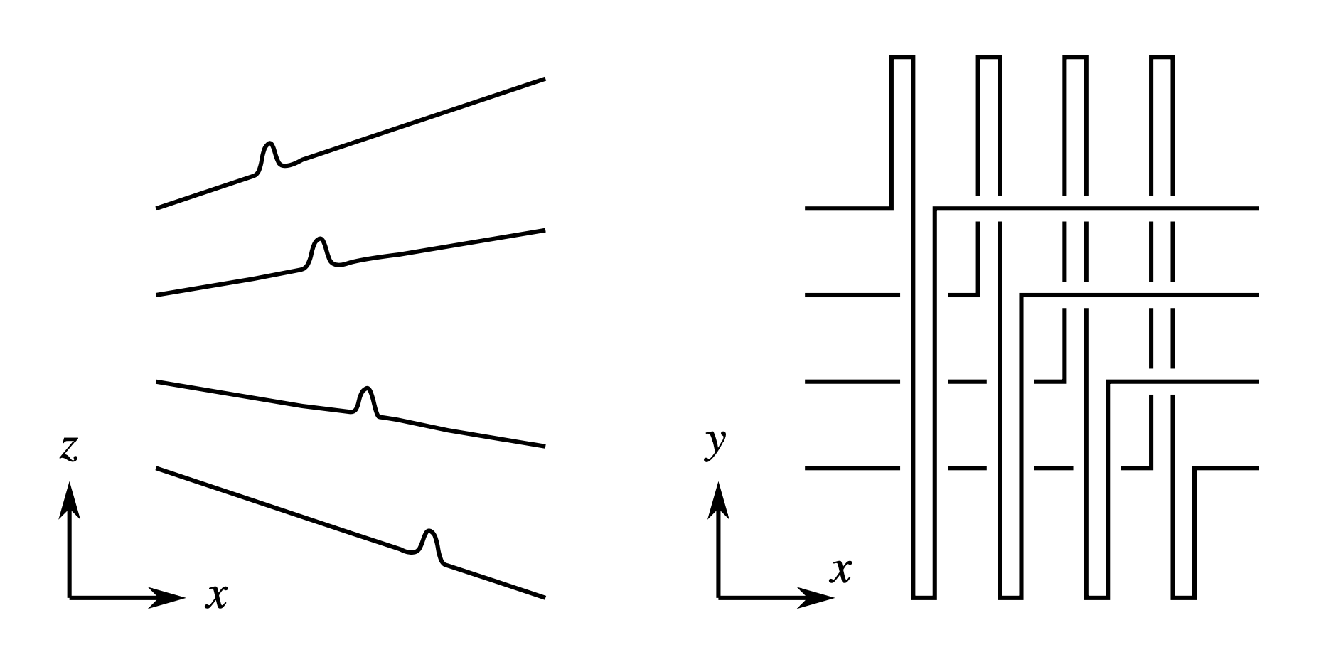
An important case is when \( M=\mathbb{R}^3 \) with its standard contact structure, \[ \xi_{\mathrm{std}} = \operatorname{ker}( dz-y\,dx) \]
(as pictured in Figure 1), where the study of Legendrian knots can be viewed as an interesting variant on the classical theory of knotted circles in 3-dimensional space. In this setting, a smooth knot \( L \subset \mathbb{R}^3 \) parametrized as \( t \mapsto (x(t),y(t),z(t)) \) is Legendrian if and only if it satisfies the differential equation \( z^{\prime}(t) = y(t) x^{\prime}(t) \). As this amounts to the identity \( y = dz/dx \), Legendrian knots in standard contact \( \mathbb{R}^3 \) are conveniently viewed via their front projections to the \( xz \)-plane since the missing \( y \)-coordinate can be recovered as the slope in this projection. Front projections of Legendrian knots are closed curves without tangential double points or vertical tangencies and having cusp singularities; see Figure 1. In the remainder of the article, unless otherwise specified, all Legendrian knots are in \( (\mathbb{R}^3, \xi_{\mathrm{std}}) \).
Two Legendrian knots are Legendrian isotopic if they are smoothly isotopic through other Legendrian knots. A similar notion of transverse isotopy exists for transverse knots and either notion is equivalent to the knots being related by an ambient contact isotopy. Note that any Legendrian knot has a well-defined underlying topological type as an ordinary (smooth) knot in \( \mathbb{R}^3 \), so that one can speak for instance of Legendrian unknots or Legendrian trefoils. A fundamental problem of Legendrian knot theory is:
The classification for Legendrian unknots was accomplished by Eliashberg and Fraser in [e11], [e31]. Around 2000, Legendrian torus knots and figure-eight knots were classified by Etnyre and Honda [e15], and subsequently complete classifications have been obtained for some additional families of topological knot types; see, e.g., [e39], [e37]. In general, the Legendrian isotopy problem remains difficult. For instance, a glance at the Legendrian Knot Atlas [e38] reveals many topological knot types with 9 or fewer crossings containing Legendrian knots that are conjectured to be distinct but have not been successfully distinguished with any known invariants.
2. The work of Fuchs and Tabachnikov
In the past decades there has been something of an explosion of work related to Legendrian knot theory. Indeed, in June 2020 MathSciNet returns 133 matches for articles containing “Legendrian” and “knot” or “link” in the title. The sixth of these to appear chronologically, and one of the most highly cited, is the article “Invariants of Legendrian and transverse knots in the standard contact space”, by D. Fuchs and S. Tabachnikov.
2.1. Stable classification
A fundamental result from
[1]
addresses a stable version of the Legendrian isotopy problem. For a
Legendrian knot, \( L \subset \mathbb{R}^3 \),
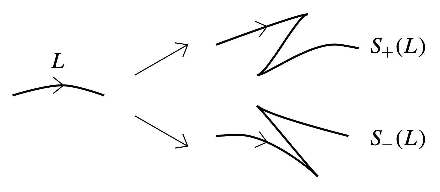
positive and negative stabilizations of \( L \),
denoted
by \( S_{+}(L) \) and \( S_-(L) \), arise from adding
zig-zags to the front projection of \( L \), as shown in
Figure 2, where the sign is determined by the whether the orientation of
the knot passes the new cusps in the downward or upward direction.
Thus, the stable Legendrian isotopy problem reduces to the isotopy problem for topological knots!1 The idea of the proof is to convert the sequence of topological knot diagrams that appear during a generic topological isotopy into front projections of Legendrian knots by adding cusps at vertical tangencies and near crossings where the over strand has larger slope. The successive topological diagrams that appear are related by Reidemeister moves and other modifications involving vertical tangencies, and it is shown that for any such bifurcation the corresponding front projections will be related by Legendrian isotopy after adding enough zig-zags.
In Theorem 2.1, it is important that stabilizations of both signs are allowed. Indeed, in the article by Epstein, Fuchs and Meyer [2] a modification of the argument from [1] is used to show that two Legendrian knots become equivalent after positive (resp. negative) stabilizations if and only if their positive (resp. negative) transverse push-offs, obtained by shifting a small amount in the positive (resp. negative) normal direction within the contact planes, are isotopic as transverse knots. As a result, the isotopy problem for transverse knots is reduced to the \( S_+ \)-stable (or \( S_- \)-stable) version of the Legendrian isotopy problem.
2.2. Bennequin-type inequalities and knot polynomials
In dimension 3, there is an opportunity for interaction between Legendrian knot theory and topological knot theory. In this direction, Fuchs and Tabachnikov observed in [1] an interesting relation between the classical invariants of a Legendrian knot and the famous HOMFLY-PT and Kauffman knot polynomials2 discovered in the 1980s. Before stating their result, let us review the context.
There are two classical integer-valued invariants of a Legendrian knot \( L \): the Thurston–Bennequin number, \( \operatorname{\mathit{tb}}(L) \), measures the linking number of \( L \) with its positive transverse push-off, and the rotation number, \( r(L) \), measures rotation of the tangent vector to \( L \) within the contact planes using a trivialization of \( \xi \). With the classical invariants in mind, a starting point for the Legendrian isotopy problem is to try to answer the following problem formulated by Eliashberg in [e6]:
By applying stabilizations, it is easy to make \( \operatorname{\mathit{tb}}(L) \) become negative with arbitrarily large magnitude without changing the topological knot type. However, for the standard (tight!) contact structure on \( \mathbb{R}^3 \) the Thurston–Bennequin number is bounded above within any fixed topological knot type. The first such upper bound appears in the seminal work of Bennequin [e1] which established the existence of a contact structure on \( \mathbb{R}^3 \) not diffeomorphic to the standard one. Bennequin proved an inequality for transverse knots that, by considering transverse push-offs, is equivalent to the statement that any Legendrian knot \( L \) in \( (\mathbb{R}^3, \xi_{\mathrm{std}}) \) satisfies \[ \operatorname{\mathit{tb}}(L) + |r(L)| \leq 2g(L)-1, \]
where \( g(L) \) is the minimum genus of any Seifert surface for \( L \). In particular, any Legendrian unknot must have \( \operatorname{\mathit{tb}} \leq -1 \). By contrast, using the contact structure \( \xi_{\mathrm{ot}} \) given in cylindrical coordinates as the kernel of the 1-form \( \cos r\, dz+ r \sin r\,d\theta \) the circle in the \( xy \)-plane centered at the origin with radius \( 2\pi \) is a Legendrian unknot with \( \operatorname{\mathit{tb}}=0 \). Thus, there is no diffeomorphism of \( \mathbb{R}^3 \) taking \( \xi_{\mathrm{std}} \) to \( \xi_{\mathrm{ot}} \). From Bennequin’s inequality, we see that there is a maximum value of \( \operatorname{\mathit{tb}} \) among Legendrian knots in any topological knot type \( \mathcal{K} \) that we will denote by \( \overline{\operatorname{\mathit{tb}}}(\mathcal{K}) \). Note that except for unknots the right-hand side of the inequality is positive, and this raises the question: are there any topological knot types with \( \overline{\operatorname{\mathit{tb}}}(\mathcal{K}) \) less than \( -1 \)?
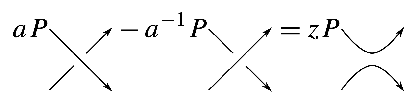
Fuchs and Tabachnikov found that inequalities of a similar flavor to Bennequin’s arise from the HOMFLY-PT and Kauffman knot polynomials, \( P_K \) and \( F_K \). These invariants assign to any topological knot \( K \) two variable Laurent polynomials, \( P_K, F_K \in \mathbb{Z}[a^{\pm1}, z^{\pm1}] \), that are characterized by simple skein relations. For instance, the HOMFLY-PT polynomial is uniquely determined by isotopy invariance, its value on the unknot which we take here to be 1, and the identity shown in Figure 3, which holds when a knot diagram is modified locally as pictured.
and \begin{equation} \operatorname{\mathit{tb}}(K) \leq - \operatorname{deg}_a F_{K}(a,z) -1, \end{equation}
where \( \operatorname{deg}_a P_K \) and \( \operatorname{deg}_a F_K \) denote the maximum degree in the variable \( a \) of the HOMFLY-PT and Kauffman polynomials.
In [1], the HOMFLY-PT inequality is observed as an immediate consequence of the combination of the works of Bennequin and Morton, Franks and Williams [e2], [e3], and the Kauffman estimate is then deduced using a nice trick involving Rudolph’s relation [e5] between the Kauffman polynomial of a knot and the HOMFLY-PT polynomial of its double with opposite orientations.3 As such, the authors of [1] elected to locate these inequalities in the background section, possibly leading to some later confusion in the literature about the origin of these inequalities.
For the left-handed trefoil, \( T \), a simple computation of the Kauffman polynomial resolves the above question, as \[ F_T(a,z) = a^2(2+z^2) -a^3z -a^4(1+z^2) + a^5z, \]
so that Theorem 2.2 gives a sharp estimate showing that \( \overline{\operatorname{\mathit{tb}}}(T) = -6 \) is indeed less than \( -1 \).4 Moreover, either of the estimates from Theorem 2.2 gives an elementary proof (perhaps the simplest) that \( (\mathbb{R}^3, \xi_{\mathrm{std}}) \) is tight and thus is distinct from \( \xi_{\mathrm{ot}} \). In later years, several additional Bennequin-type inequalities have been discovered with quantities derived from various topological knot invariants appearing on the right-hand side. See [e29] for the state of the art circa 2008, as well as [e10], [e36], [e40] for extensions of Theorem 2.2 to some other ambient contact manifolds.
2.3. Legendrian simplicity and finite-type invariants
To complement the Legendrian geography problem, it is natural to ask to what extent the classical invariants determine Legendrian (or transverse) knot types.5 In this direction, call a topological knot type Legendrian (or transversally) simple if any two Legendrian (or transverse) knots within the knot type that have equal classical invariants are Legendrian (or transverse) isotopic. At the time [1] was written, it was not known whether any knot types in \( (\mathbb{R}^3, \xi_{\mathrm{std}}) \) were nonsimple in either the Legendrian or transverse sense.6 One way to produce examples of Legendrian knots with the same classical invariants and underlying knot type is by the Legendrian mirror operation that takes \( L \) to its image \( L^\vee \) under the diffeomorphism of \( \mathbb{R}^3 \) that maps \( (x,y,z) \mapsto (x,-y,-z) \). See Figure 4. In general, \( \operatorname{\mathit{tb}}(L^\vee) = \operatorname{\mathit{tb}}(L) \) and \( r(L^\vee) = -r(L) \), so when \( r(L) =0 \) the classical invariants are unchanged leading to the following problem formulated by Fuchs and Tabachnikov in [1].
At the time, the central difficulty in finding examples of non-Legendrian simple knot types was that no Legendrian invariants beyond \( \operatorname{\mathit{tb}} \) and \( r \) were known to exist. One of the main results of [1], which uses a natural extension of the class of finite-type knot invariants (see, e.g., [e8]) to the setting of Legendrian and transverse knots, elucidates the difficulty of finding such invariants and could even be viewed as evidence that such invariants might not exist.7
This theorem was later extended to Legendrian knots in a much wider class of contact manifolds, including all tight contact structures, in the work of V. Tchernov [e18]. Interestingly, Tchernov also finds examples of knots in overtwisted contact structures on \( S^1\times S^2 \), where a statement analogous to that of Theorem 2.3 no longer holds!
3. New invariants and normal rulings
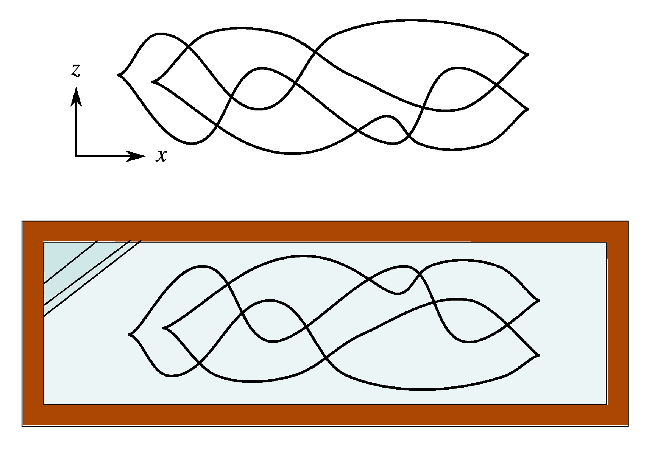
In the late 1990s a major development occurred in Legendrian knot theory with the discovery8 of the Chekanov–Eliashberg algebra, a new invariant capable of distinguishing between Legendrian knots with the same classical invariants. This invariant is a differential graded algebra (abbreviated DGA) arising from \( J \)-holomorphic curve theory that can be formulated in an entirely combinatorial manner. In its initial version,9 the DGA assigned to a Legendrian knot \( L \) consists of a free associative (but noncommutative) \( \mathbb{Z}/2\mathbb{Z} \)-algebra, \( \mathcal{A}(L) \), generated by the double points of \( L \) under the Lagrangian projection, \( \pi_{xy}:\mathbb{R}^3 \rightarrow \mathbb{R}^2 \), \( (x,y,z) \mapsto (x,y) \), together with a differential \( \partial: \mathcal{A}(L) \rightarrow \mathcal{A}(L) \) defined by a count of immersed polygons in the plane with boundary on \( \pi_{xy}(L) \). A \( \mathbb{Z}/2r(L)\mathbb{Z} \)-grading, which proves crucial in many applications, arises from the rotation numbers of certain capping paths for crossings of \( \pi_{xy}(L) \). In his famous article [e16], Chekanov applied the DGA to distinguish a pair of \( m(5_2) \) knots with the same classical invariants, establishing the first example of a Legendrian nonsimple knot type. As another early application, in [e19] Lenny Ng made use of the noncommutativity of the Chekanov–Eliashberg DGA to resolve the Legendrian mirror problem by exhibiting a Legendrian \( 6_2 \) knot, pictured in Figure 5, with zero rotation number that is not equivalent to its Legendrian mirror.10
3.1. Augmentations and normal rulings
Fuchs was an early proponent of the Chekanov–Eliashberg DGA, as he explored and applied this invariant in a sequence of articles several of which were coauthored with grad students at UC Davis. The Chekanov–Eliashberg DGA is somewhat unwieldy to work with in its entirety as the graded pieces of \( \mathcal{A}(L) \) and also of its homology tend to be infinite-dimensional. One way to obtain easily computable invariants, used initially by Chekanov, is to employ an augmentation of \( \mathcal{A}(L) \) which is an algebra map \( \epsilon: \mathcal{A}(L) \rightarrow \mathbb{Z}/2\mathbb{Z} \) that satisfies \( \epsilon \circ \partial = 0 \), \( \epsilon(1) =1 \), and preserves grading. When \( \mathcal{A}(L) \) has an augmentation, the DGA can be linearized to produce a finite-dimensional chain complex whose homology can be used for distinguishing Legendrian knots. For instance, in [2] Epstein, Fuchs, and Meyer establish the existence of augmentations for a family of Legendrian twist knots, referred to there as Eliashberg knots, and are then able to effortlessly distinguish these knots from one another using only the degree distribution of crossings.11 An important question then becomes:
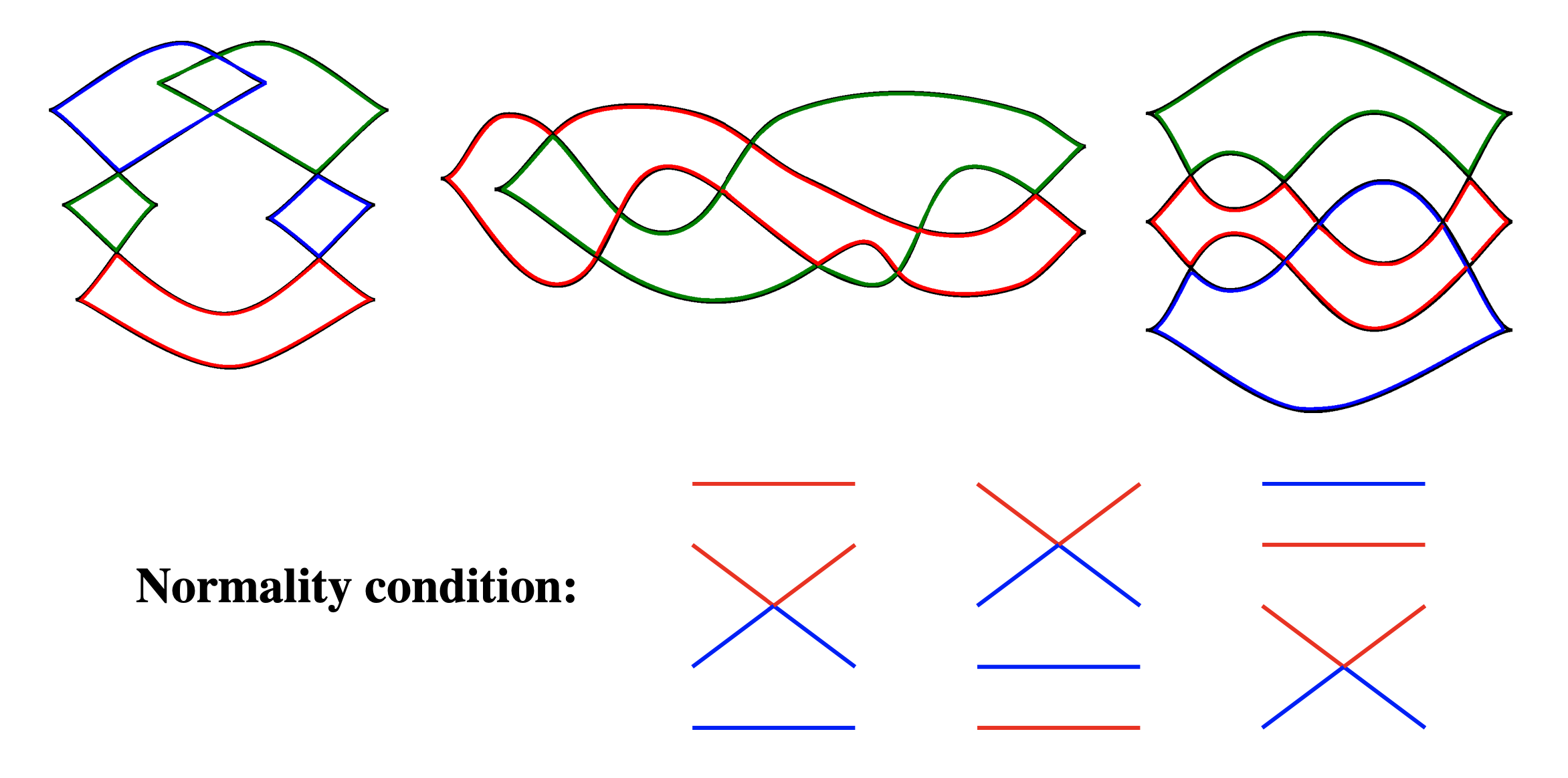
In investigating this question, Fuchs discovered in [3] a beautiful combinatorial structure arising in the front projections of Legendrian knots called a normal ruling. For a Legendrian link \( L \) in \( \mathbb{R}^3 \), a normal ruling is a decomposition of the front projection of \( L \) into a collection of simple closed curves, each of which has corners at a left and right cusp, and at some subset of the crossings called “switches”; see Figure 5. The decomposition is subject to certain restrictions, including the normality condition illustrated in Figure 5. Given a divisor, \( \rho \,|\, 2 r(L) \), a normal ruling is said to be \( \rho \)-graded if all crossings that are switches have their degrees congruent to 0 mod \( \rho \). One can also consider \( \rho \)-graded augmentations by weakening the grading requirement so that \( \epsilon:\mathcal{A}(L) \rightarrow \mathbb{Z}/2 \) only needs to preserve grading mod \( \rho \). Often 1-graded normal rulings or augmentations are referred to as ungraded since when \( \rho=1 \) the grading condition becomes vacuous.
The forward direction was established in [3], while the reverse implication was proven independently by Fuchs and Ishkhanov [5] and Sabloff [e21]. For the proof, in [3] Fuchs introduced an elegant method of adding “splashes” via a Legendrian isotopy in order to greatly simplify the differential at the expense of adding many additional generators to \( \mathcal{A}(L) \). Fuchs’ splashes appear as little ripples in the front projection that become steep waves when viewed in the Lagrangian projection. As a result the holomorphic disks that contribute to the differential of \( (\mathcal{A}(L), \partial) \) become trapped in thin vertical strips between successive pairs of splashes. This results in explicit matrix formulas for differentials depending only on the local appearance of \( L \) between two splashes, which may be taken to consist of a single crossing or cusp.12
Interestingly, the notion of normal ruling was discovered independently by Chekanov and Pushkar in a somewhat different context.13 In [e20] they introduced normal rulings, under the name of positive proper decompositions, in the context of generating families for Legendrian knots, and applied properties of the behavior of normal rulings under generic Legendrian isotopies in their solution of the Arnold 4-conjectures.14 A generating family (of functions) for a Legendrian knot \( L \) in \( \mathbb{R}^3 \) is a one-parameter family of functions \( \{f_x\}_{x \in \mathbb{R}} \) whose critical values trace out the front projection of \( L \). Generating families are a standard tool in symplectic topology, and they were applied in the work of Traynor [e14] to distinguish certain two-component Legendrian links with the same classical invariants. In influential but unpublished work, Pushkar had also suggested a method for defining a Legendrian homology using generating families as well as a combinatorial approach to the whole theory via what M. B. Henry would call Morse complex sequences in his thesis [e32]. As (i) Chekanov and Pushkar had shown that (linear at infinity) generating families for \( L \) exist if and only if \( L \) has a normal ruling, and (ii) Pushkar’s generating family homology could be computed using a complex generated by the crossings of \( \pi_{xy}(L) \), it seemed likely that there would be a connection between generating families and augmentations.
In [6], Fuchs and I established such a connection by constructing an augmentation from a generating family and providing an isomorphism between the corresponding linearized homology and generating family homology groups. Under this isomorphism, Sabloff’s duality result [e28] for the linearized homology groups of the Chekanov–Eliashberg algebra appears on the generating family side as the Alexander duality. The idea for constructing an augmentation, \( \epsilon \), from a generating family, \( \{f_x\} \), is to again work with a splashed version of \( L \). Then, the generators of \( \mathcal{A}(L) \) can be collected together in a sequence of matrices \( X_1, \ldots, X_r \) and \( Y_1, \ldots, Y_r \) associated to the different splashes located at a sequence of \( x \)-values \( x_1 < x_2 < \cdots < x_r \). One then uses the generating family to define an augmentation, \( \epsilon \), by taking \( \epsilon(Y_i) \) to be the matrix of the differential in the Morse complex of \( f_{x_i} \) and \( \epsilon(X_i) \) to be the matrix of a continuation map between the Morse complexes of \( f_{x_i} \) and \( f_{x_{i+1}} \). The linearized homology complex associated to \( \epsilon \) then corresponds to the generating family homology via a cellularization by fiberwise descending/ascending manifolds that was also known to Pushkar as a means for computing the generating family homology.
3.2. Fuchs’ “irresponsible conjecture”
In the article [3] where he introduced normal rulings, Fuchs made an elegant conjecture connecting the new Legendrian invariants with topological knot theory.
The conjecture was based on a study of mirror torus knots in [4] and evidence from knots with small crossing number. Despite being dubbed “irresponsible” in [3], the conjecture turned out to be completely accurate and was proven in [e25] as a consequence of a more precise relationship between normal rulings and the Kauffman polynomial. In [e20], Chekanov and Pushkar had obtained Legendrian invariants by making a refined count of normal rulings: they showed that for any \( n \in \mathbb{Z} \) and \( \rho \,|\, 2 r(L) \), the number, \( f^\rho_n \), of \( \rho \)-graded normal rulings, \( \sigma \), of \( L \) with \[ j(\sigma) := \#\,\mbox{switches} - \#\,\mbox{right cusps} \]
equal to \( n \) is a Legendrian isotopy invariant of \( L \). With \( \rho \) fixed, it is convenient to collect these numbers as the coefficients of a \( \rho \)-graded ruling polynomial defined by summing over all \( \rho \)-graded normal rulings for \( L \) as \[ R_L^\rho(z):= \sum_{\sigma} z^{j(\sigma)} = \sum_{n\in \mathbb{Z}} f^\rho_{n}z^n. \]
The 0-graded ruling polynomial can distinguish knots with the same classical invariants, such as Chekanov’s pair of \( m(5_2) \) knots. In contrast, when \( \rho =1 \) or 2 the ruling polynomial depends only on \( \operatorname{\mathit{tb}} \) and the underlying topological knot type as shown by the following.
To see that Fuchs’ conjecture follows as a corollary, observe that the inequality (1) is sharp if and only if the coefficient of \( a^{-\operatorname{\mathit{tb}}(L)-1} \) in \( F_L \) is nonzero. Since this coefficient is the ungraded ruling polynomial, \( R^1_L(z) \), it is nonzero if and only if \( L \) has an ungraded normal ruling and this is equivalent by Theorem 3.2 to \( \mathcal{A}(L) \) having an ungraded augmentation.
The connection between normal rulings, augmentations of the Chekanov–Eliashberg algebra, and the topological knot polynomials has been strengthened in several subsequent works. Building on the many-to-one correspondence between augmentations and normal rulings over \( \mathbb{Z}/2\mathbb{Z} \) from [e26] and Henry’s study of augmentations and Morse complex sequences from [e32], Henry and I showed in [e43] that the ruling polynomials specialized at \( z= q^{1/2}-q^{-1/2} \) with \( q \) a prime power correspond to counts of augmentations of \( \mathcal{A}(L) \) to finite fields \( \mathbb{F}_q \) and in this way are determined by the Chekanov–Eliashberg DGA. The works [e41], [e44], [e45] relate counts of higher-dimensional representations of \( \mathcal{A}(L) \) to ruling polynomials of Legendrian satellites and (when \( \rho = 1 \) or 2) to the \( n \)-colored Kauffman and HOMFLY-PT polynomials. Precisely how much of the DGA \( (\mathcal{A}(L), \partial) \) is determined by the Thurston–Bennequin number and topological type of \( L \) remains an interesting question, and some open conjectures on this topic appear in [e19], [e41].
4. Working with Fuchs at UC Davis
Having Dmitry Fuchs as an advisor at UC Davis was a privilege and a pleasure. I came into contact with Dmitry, whom I always referred to as Dr. Fuchs while I was a student, as soon as classes started upon my arrival at UC Davis in 2003 as he taught the first two thirds of the year-long algebra sequence for new Ph.D. students. The topics covered by Fuchs in the course were linear algebra, rings and modules, category theory, and Galois theory. Homological algebra was covered in the final third of the course sequence, taught that year by Dmitry’s own advisor, Albert Schwarz. I particularly enjoyed the exercises Fuchs had assembled for the class, from which students were allowed to choose from an ample selection of problems which pulled in many additional topics, especially in the category theory part of the class.
As the first year wrapped up, in order to receive summer support from UC Davis’ VIGRE grant I needed to work on a research project. But, I had no research program. What to do? With another student, Chris Berg, we decided to talk to Fuchs who agreed to supervise a summer project, and helped us to quickly write a proposal. Although the proposal had involved characteristic classes of families of foliations, leading me to scramble to assemble some background in differentiable manifolds which I did not have at the time, during the summer Dmitry shared his conjecture about normal rulings and the Kauffman polynomial. Following Dmitry’s suggestions, we established the sharpness of the estimate (1) for several families of Legendrian knots constructed so that their front diagrams would have obvious normal rulings.
After the summer, Chris turned his interests toward combinatorial representation theory and began working with M. Vazirani, going on to do excellent work in this area. I continued to work with Dr. Fuchs, and as I attended his year-long algebraic topology course,15 we started weekly meetings that would continue off and on for the rest of my time at UC Davis. During these meetings, which often took place at Dmitry’s home office and could last for 2 to 3 hours, Dmitry was extremely generous with his time and knowledge. As a result, I was exposed to a variety of Dmitry’s (many) favorite topics including Lie algebra cohomology and foliations, evolutes and involutes of plane curves, contact and symplectic topology, representations of the Virasoro algebra, singular vectors in Verma modules of affine Lie algebras, etc. Dmitry has a particular affinity for (and encyclopedic knowledge of!) classical algebraic topology, and a question about K-theory or spectral sequences could lead to a two-hour improvised overview of the topic.
I was still somewhat hooked on the problem about normal rulings and the Kauffman polynomial and from time to time would come back to it and expand the class of examples for which I could prove Fuchs’ conjecture. A particular exciting day of mathematics for me resulted after reading about Chekanov and Pushkar’s ruling invariant in the paper [e26] of Ng and Sabloff, formulated there as a multiset of integers, i.e., a finite sequence of nonnegative integers. On the bike ride home I started thinking about the top degree of the Kauffman polynomial, the part that needs to be nonzero in order for the estimate to be sharp. It’s also a sequence of integers (but nonnegative?). What if it was the same sequence? I had a pretty good idea in my head of what the Kauffman polynomial of the trefoil looked like, and that seemed to check out. Once I got home, I checked the figure-eight knot. As it can be a little tricky to identify all of the normal rulings of a front projection by hand, I sat down and wrote a C++ program to compute the ruling invariant and then started comparing the results with the tables of the Kauffman polynomial one knot at a time. Except for some signs in the coefficients of the Kauffman polynomial, each and every knot worked out exactly!!!16 I was excited to tell Dr. Fuchs the news. At the start of our next meeting I let him know that I had made an interesting discovery. Dmitry’s response, with a bit of twinkle in his eye, was “I like interesting discoveries…” He handed me the pen. After understanding my refinement of his conjecture and checking it for a few knots, Dmitry was visibly excited. He immediately adjourned the meeting saying that he had some other topics that he had planned to discuss with me but now it did not seem so important. I left his house under orders to begin writing a paper with the special cases that I was able to prove. On the way home I can remember pausing on a hill in a park and feeling satisfied and excited in the perfect Davis summer weather.
With the more specific statement in hand, the conjecture was not hard to prove. Viewing the ruling invariant as a knot polynomial, I soon realized a version of its skein relation using a local picture with two cusps. But, it seemed too specific to be applicable to arbitrary Legendrian knots. Later in my office I saw that a more general skein relation held and checked through the case-by-case inductive argument that showed that the skein relation, also satisfied by the top term of the Kauffman polynomial, would uniquely characterize a Legendrian invariant. I sent Dmitry a quick e-mail letting him know that his conjecture could now be considered a theorem. It was exciting to know that the result was true!
By generously sharing his conjecture and other problems with me, Dmitry gave me the chance to enter the mathematical research community, but his support did not end there. After finishing my Ph.D. at UC Davis, Dmitry helped me to obtain valuable post-doc positions at Duke University where I worked with Lenny Ng and later at University of Arkansas where I worked with Yo’av Rieck. Moreover, he helped me to make important connections with other researchers interested in Legendrian knots and related topics by, not long after I completed my Ph.D., organizing with S. Tabachnikov and L. Traynor a workshop at AIM. This workshop also resulted in an offshoot SQuaREs group that stimulated my collaboration with Brad Henry. Dmitry also encouraged me to travel internationally, and in particular to spend a productive and enjoyable month at MPIM in Bonn.
Thank you, Dmitry! I am truly grateful to you for sharing your knowledge and joy in doing mathematics and for all of your help along the way!
The author is an Associate Professor at Ball State University in Muncie, Indiana. He enjoys spending time with family and grooving to the sounds of classic jazz from the 1950s and 60s.
