by Leonid Polterovich and Felix Schlenk
In this essay we describe some of Dusa’s contributions to symplectic embedding problems. Let us first say what these problems are about: A symplectic manifold \( (M,\omega) \) is a smooth manifold \( M \) together with a closed and nondegenerate differential two-form \( \omega \). The dimension must then be even. Examples are Kähler manifolds and cotangent bundles \( T^*Q \) with their canonical symplectic form \[ \sum_{i=1}^n dq_i \wedge dp_i ,\]
in which Hamiltonian mechanics takes place. The time-1 map \( \varphi \) of a Hamiltonian flow on \( (M,\omega) \) preserves the symplectic form: \( \varphi^*\omega = \omega \). Any map with this property is called symplectic. The study of symplectic mappings thus gives insight into the possible dynamics of a classical mechanical system.
Every symplectic manifold locally looks like \( \mathbb{R}^{2n} \) with the constant symplectic form \[ \omega_0 = \sum_{i=1}^n dx_i \wedge dy_i .\]
It is thus already interesting to study symplectic mappings between open subsets \( U \), \( V \subset \mathbb{R}^{2n} \). Every symplectic mapping is a local embedding; but looking at all symplectic mappings is not interesting, for instance all of \( \mathbb{R}^{2n} \) can be symplectically immersed into a tiny ball. On the other hand, deciding when two open subsets are symplectically diffeomorphic turns out to be too hard in general. To learn something interesting, one looks at the intermediate problem of symplectic embeddings. We write \( U \stackrel{s}{\hookrightarrow} V \) if there exists a symplectic embedding \( U \hookrightarrow V \). In this case, \( \operatorname{Vol} (U) \leqslant \operatorname{Vol} (V) \), since symplectic diffeomorphisms preserve the volume \[ \operatorname{Vol} (U) = \frac{1}{n!} \int_U \omega^n .\]
We assume throughout that \( 2n \geqslant 4 \), since two-dimensional symplectic mappings are just those that preserve the area and the orientation. Also note that \( U \stackrel{s}{\hookrightarrow} V \) if and only if \( \lambda U \stackrel{s}{\hookrightarrow} \lambda V \) for every \( \lambda > 0 \).
Denote by \( \operatorname{B}^{2n}(a) \) the open ball in \( \mathbb{R}^{2n} \) of “area” \( a = \pi r^2 \), where \( r \) is the radius, and by \( \operatorname{Z}^{2n} \) the full cylinder \[ \operatorname{B}^2(1) \times \mathbb{R}^{2n-2} \quad\text{in}\quad \mathbb{R}^2(x_1,y_1) \times \mathbb{R}^{2n-2}(x_2, y_2, \dots, x_n,y_n) .\]
The starting point of the symplectic embedding story is Gromov’s nonsqueezing theorem [e1]: \[ \operatorname{B}^{2n}(a) \stackrel{s}{\hookrightarrow} \operatorname{Z}^{2n} \quad\mbox{only if}\quad a \leqslant 1. \]
In other words, the inclusion \( \operatorname{B}^{2n}(1) \subset \operatorname{Z}^{2n} \) is already “the best” symplectic embedding! There are (even linear) volume preserving embeddings of \( \operatorname{B}^{2n}(a) \) into \( \operatorname{Z}^{2n} \) for any \( a > 1 \). Symplectic mappings are thus much more rigid than volume preserving mappings, i.e., the evolutions in Hamiltonian dynamics are much more constraint than those in ergodic theory. The key in Gromov’s proof is the existence of a suitable \( J \)-holomorphic sphere in the partial compactification \( S^2 \times \mathbb{R}^{2n-2} \) of \( \operatorname{Z}^{2n} \).
The starting point of our discussion is the following problem, which demonstrates both rigid and flexible behaviour of symplectic mappings: fill as much as possible of \( \operatorname{B}^4(1) \) by \( k \) symplectically embedded equal balls \( \operatorname{B}^4(a) \).
Let \( p_k \) be the percentage of the volume of \( \operatorname{B}^4(1) \) that can be filled by \( k \) symplectically embedded equal balls. Then \( p_k \) has the following values: \[ \begin{array}{c|ccccccccc} \hline k & 1 & 2 & 3 & 4 & 5 & 6 & 7 & 8 & \geqslant 9 \\ \hline p_k & 1 & \dfrac 12 & \dfrac{3}{4} & 1 & \dfrac{20}{25} & \dfrac{24}{25} & \dfrac{63}{64} & \dfrac{288}{289} & 1 \\ \hline \end{array} \]
The inequalities \( p_2 \leqslant 1/2 \) and \( p_5 \leqslant 4/5 \) were found by Gromov [e1] as an application of his theory of pseudoholomorphic curves in symplectic manifolds. Gromov’s discovery was that the algebraic geometry of curves in complex manifolds to a high extent extends to curves in almost-complex manifolds provided that the almost complex structure is compatible with a symplectic form. In particular, the Gromov–Euclid theorem states that, under the compatibility assumption, through every pair of points in any almost-complex projective plane passes a unique line. Given a symplectic packing of \( \operatorname{B}^4(1) \) by two balls, \( B_1 \) and \( B_2 \) of radius \( r \), compactify \( \operatorname{B}^4(1) \) to \( \operatorname{\mathbb{C}P}^2 \) and change the complex structure on \( \operatorname{\mathbb{C}P}^2 \) to a compatible almost complex structure \( J \) which is standard on \( B_1 \) and \( B_2 \). Take a \( J \)-holomorphic line \( L \) passing through the centers of the balls. By Lelong’s inequality, \[ \operatorname{Area}(L \cap B_i) \geqslant \pi r^2 .\]
On the other hand, the total area of \( L \) equals \( \pi \), which readily yields \( 2\pi r^2 \leqslant \pi \) and hence \( p_2 \leqslant 1/2 \).
In the summer of 1991, both Dusa and Leonid visited Helmut Hofer in Bochum. Helmut suggested Leonid to work on the concept of super-recurrence in Hamiltonian dynamics: indeed, symplectic maps tend to have more periodic orbits than general volume preserving maps. Leonid’s take on the problem was as follows: assume that for some \( k \) we have \( p_k < 1 \). This means that \( \operatorname{\mathbb{C}P}^2 \) cannot be fully packed by \( k \) balls of volume \( \operatorname{Vol}(\operatorname{\mathbb{C}P}^2)/k \). In particular, if \( B \) is such a ball and \( \varphi \) is any symplectomorphism of \( \operatorname{\mathbb{C}P}^2 \), one of the sets \( \varphi^j(B) \), \( j=1,\dots \), \( k-1 \) must intersect \( B \). This constraint, which is specific to symplectic maps, can be interpreted as a short term super-recurrence. To have a long term super-recurrence, one wants to have inequalities \( p_k < 1 \) for an infinite number of values of \( k \) (a few years later Paul Biran showed that this is not the case, see below). This gave rise to the following question: why did Gromov stop at \( k=5 \) balls, the case based on studying conics passing through 5 points? An analysis showed that for large \( k \), the upper bound for \( p_k \) based on Gromov’s \( J \)-holomorphic curves of higher degree is useless: it exceeded 1! (Later on, Misha Gromov remembered that it was David Kazhdan who warned him about the large \( k \) case). What happens in between, i.e., for which values of \( k \) do pseudoholomorphic curves beat the trivial volume-based estimate? Dusa and Leonid were intrigued and decided to explore. At that time Dusa had already introduced the technique of symplectic blowing up, a fundamental construction going back to Gromov and Guillemin–Sternberg, into symplectic topology [1]: Given an embedding \[ \varphi \colon \operatorname{B}^4(a)\stackrel{s}{\hookrightarrow} \operatorname{B}^4(1) ,\]
one removes \( \varphi (\operatorname{B}^4(a)) \) and collapses the remaining boundary along the characteristic foliation, which is given by the orbits of the Hopf-flow on the 3-sphere. This technique became the main tool in the paper of McDuff and Polterovich [2], which settled the above table for \( k \leqslant 8 \). Let us retell Gromov’s proof of \( p_2 \leqslant 1/2 \) in the language of blow-ups. Given a packing of \( \operatorname{\mathbb{C}P}^2 \) by balls of radius \( r \), one can blow them up and get the del Pezzo surface \( M \) such that the area of the general line \( L \) is still \( \pi \), while the areas of the exceptional divisors \( E_1 \) and \( E_2 \) equal \( \pi r^2 \). One checks that the class \( L-E_1-E_2 \) corresponding to the proper transform of the Gromov–Euclid line is exceptional, i.e., has self-intersection \( -1 \), and hence, by an earlier result of Dusa, is represented by a pseudoholomorphic curve. Its area \( \pi-2\pi r^2 \) is thus positive, and so we get \( p_2 < 1/2 \). The advantage of this approach is that it generalizes to \( k \leqslant 8 \), and the packing inequalities for \( k \leqslant 8 \) balls follow from the beautiful classical classification of exceptional curves on del Pezzo surfaces.
On a more personal note, I (Leonid) competed for Dusa’s attention with her son Thomas, at that time a young child who accompanied Dusa on her trip to Bochum. Dusa skillfully handled the case. Thus I got two private lessons for the price of one: not only in symplectic topology, but also in wise and very patient parenting. I use this occasion to express my gratitude and admiration to Dusa for both of them.
\( J \)-holomorphic curves do not yield nontrivial packing constraints for \( k \geqslant 9 \) balls. In fact it was observed in [2] that no such constraints exist (i.e., \( p_k=1 \)) modulo an old conjecture by Nagata in enumerative algebraic geometry, which in turn was motivated by Hilbert’s 14th problem. While Nagata’s conjecture is, to the best of our knowledge, still open, the packing puzzle was resolved in the PhD thesis by Paul Biran [e4], who succeeded to prove \( p_k=1 \) for \( k \geqslant 10 \) by a different method. Biran’s ingenious argument involved the symplectic inflation construction of Lalonde and McDuff [4] combined with Taubes–Seiberg–Witten theory, which he learned from an early version of Dusa’s paper [5]. In fact, flexibility of packings by a sufficiently large number of equal balls holds for every closed symplectic four manifold, as was shown by Biran [e5] for rational symplectic forms and in general very recently by Olga Buse, Richard Hind and Emmanuel Opshtein [e14].
The above packing obstructions for \( k=2,3 \), \( 5,6 \), \( 7,8 \) balls are sharp. Dusa and Leonid proved this in a highly nonconstructive way by using the Nakai–Moishezon criterion in algebraic geometry. This gave rise to the problem of explicit packing constructions. For \( k=2,3 \) balls they were found by Yael Karshon in her appendix [e2] to [2]. Later on Lisa Traynor [e3] constructed optimal packings for 5 and 6 balls, and Ingo Wieck [e7] in his PhD thesis written under the supervision of Hansjörg Geiges settled the remaining case of 7 and 8 balls. The case of \( k=m^2 \) balls is easy: use symplectic polar coordinates to represent a symplectic ball as the product of the square and the simplex, and chop the square into \( m^2 \) equal squares. This argument immediately extends to any dimension \( 2n \) for \( k=m^n \).
For symplectic packings of a ball by equal balls in higher dimensions \( 2n \), Gromov’s two ball packing theorem still works and yields sharp answers for \( k \leqslant 2^n \) balls, but the rest of the methods in [2] fails for \( 2n \geqslant 6 \). To make progress, we need to make a detour through packings by more general collections of balls and by ellipsoids.
The papers [1], [2] also contained the first step to the following algebraic reformulation of the general ball packing problem \begin{equation} \label{e:Bai} \bigsqcup_{i=1}^k \operatorname{B}^4(a_i) \stackrel{s}{\hookrightarrow} \operatorname{B}^4(A) \end{equation}
that in its full form was established by Biran, Li–Li and Li–Liu: An embedding \eqref{e:Bai} exists if and only if
(Volume constraint) \( \sum_i a_i^2 \leqslant A^2 \);
(Constraint from exceptional spheres) \( \sum_i a_i m_i \leqslant A d \) for every vector of nonnegative integers \( (d \); \( m_1, \dots \), \( m_k) \) that solves the Diophantine system \begin{equation} \label{eq:ee} \sum_i m_i = 3d-1, \qquad \sum_i m_i^2 = d^2+1 \end{equation}
and can be reduced to \( (0 \); \( -1,0,\dots \), \( 0) \) by repeated Cremona moves.
Here, a Cremona move takes a vector \( (d \); \( m_1, \dots \), \( m_k) \) with \( m_1 \geqslant \dots \geqslant m_k \) to the vector \[ (d^{\prime}; \mathbf{m}^{\prime}) = (d + \delta; \, m_1+\delta, m_2+\delta, m_3+\delta, m_4, \dots, m_k) ,\]
where \( \delta = d - (m_1+m_2+m_3) \), and then reorders \( \mathbf{m}^{\prime} \).
After a break of ten years, Dusa returned to symplectic embeddings in [6], in which she studied the problem \[ \operatorname{E} (a,b) \stackrel{s}{\hookrightarrow} \operatorname{E}(c,d) ,\]
where \[ \operatorname{E} (a,b) = \biggl\{ (z_1, z_2) \in \mathbb{C}^2 \biggm| \frac{\pi |z_1|^2}{a} + \frac{\pi |z_2|^2}{b} < 1 \biggr\} \]
is the ellipsoid in \( \mathbb{C}^2 \) whose projections to the coordinate planes are discs of area \( a \) and \( b \). Back then is was not quite clear why this is an interesting problem, but like many of Dusa’s works this paper initiated much progress on symplectic embeddings. We here assume that the target ellipsoid is a ball, that we again compactify to \( \operatorname{\mathbb{C}P}^2 \). Given an embedding \[ \varphi \colon \operatorname{E}(a,b) \stackrel{s}{\hookrightarrow} \operatorname{B}^4 \subset \operatorname{\mathbb{C}P}^2 ,\]
one can still blow-up its image, namely remove \( \varphi (\operatorname{E}(a,b)) \) and collapse the remaining boundary along the characteristic foliation, but one then obtains an orbifold instead of a manifold. It looks difficult to use \( J \)-holomorphic curves in such a space. But Dusa went around all singularities by using a version of the Hirzebruch–Jung resolution of singularities, and inflated along chains of \( J \)-spheres to reduce the problem \[ \operatorname{E}(1,a) \stackrel{s}{\hookrightarrow} \operatorname{B}^4(A) \]
to the problem \eqref{e:Bai}: \begin{equation} \label{e:equiv} \operatorname{E}(1,a) \stackrel{s}{\hookrightarrow} \operatorname{B}^4(A) \quad\Longleftrightarrow\quad \bigsqcup_{i=1}^k \operatorname{B}^4(a_i) \stackrel{s}{\hookrightarrow} \operatorname{B}^4(A) \end{equation}
where for rational \( a \) the \( a_i \) are given by \[ (a_1, \dots, a_k) =: \mathbf{w} (a) = (\underbrace{1,\dots,1}_{\ell_0}, \underbrace{w_1,\dots,w_1}_{\ell_1}, \dots, \underbrace{w_N,\dots,w_N}_{\ell_N} ) \]
with the weights \( w_i > 0 \) such that \( w_1 = a-\ell_0 < 1 \), \( w_2 = 1-\ell_1 w_1 < w_1 \), and so on. For instance, \( \mathbf{w} (3) = (1 \), \( 1,1) \) and \[ \mathbf{w} \bigl(\tfrac{11}{4}\bigr) = \bigl( 1,1, \tfrac 34, \tfrac 14, \tfrac 14, \tfrac 14 \bigr). \]
In particular, \[ \operatorname{E}(1,k) \stackrel{s}{\hookrightarrow} \operatorname{B}^4(A) \quad\text{if and only if}\quad \bigsqcup_k \operatorname{B}^4(1) \stackrel{s}{\hookrightarrow}\operatorname{B}^4(A) .\]
The ball packing problem \[ \bigsqcup_k \operatorname{B}^4(1) \to \operatorname{B}^4(A) \]
is thus included in the 1-parametric problem \[ \operatorname{E}(1,a) \stackrel{s}{\hookrightarrow} \operatorname{B}^4(A) !\]
This latter problem is encoded in the function \[ c(a) \colon [1,\infty) \to [1, \infty) \]
defined by \[ c(a) = \inf \bigl\{ A \bigm| \operatorname{E} (1,a) \stackrel{s}{\hookrightarrow} \operatorname{B}^4(A) \bigr\}. \]
For the description of \( c(a) \), recall that the Fibonacci numbers are recursively defined by \[ f_{-1}=1,\quad f_0=0,\quad f_{n+1} = f_n + f_{n-1} .\]
Denote by \( g_n: = f_{2n-1} \) the odd-index Fibonacci numbers, \[ (g_0, g_1, g_2, g_3, g_4,\dots ) = (1,1,2,5,13,\dots) .\]
The sequence \( \gamma_n := g_{n+1}/{g_n} \), whose first terms are \[ ( \gamma_0, \gamma_1, \gamma_2, \gamma_3, \dots ) = \bigl( 1, 2, \tfrac 52, \tfrac{13}{5}, \dots \bigr) , \]
converges to \( \tau^2 \), where \( \tau := (1+\sqrt{5})/2 \) is the golden ratio.
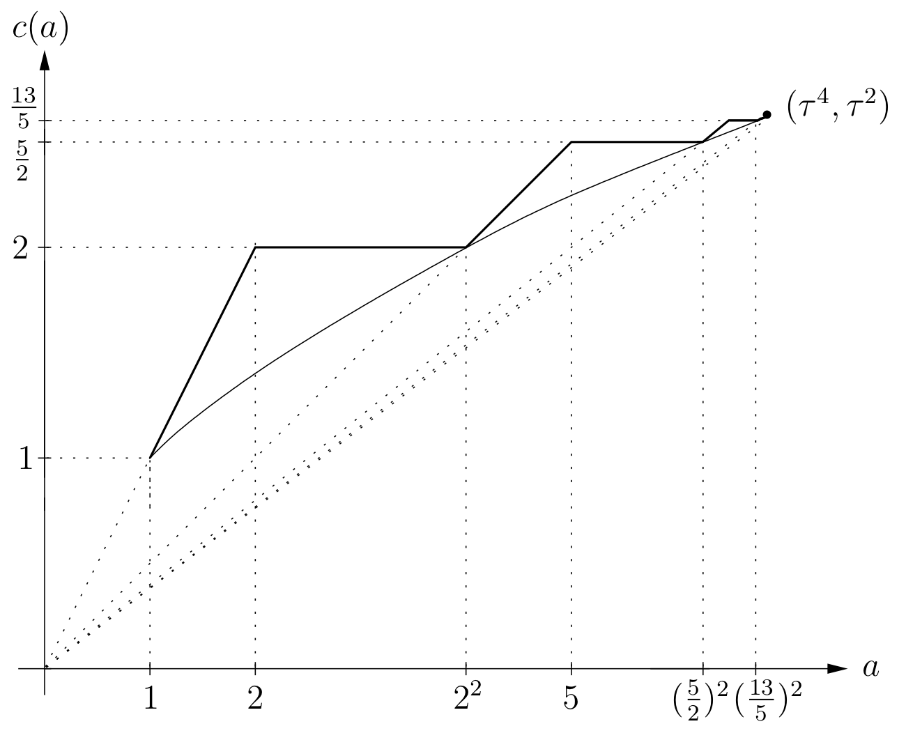
Define the Fibonacci stairs as the graph on \( [1,\tau^4] \) alternatingly formed by horizontal segments \( \{ a = \gamma_n \} \) and slanted segments that extend to a line through the origin and meet the previous horizontal segment on the graph \( \sqrt a \) of the volume constraint (the first horizontal segment has zero length), see the figure. The coordinates of all the nonsmooth points of the Fibonacci stairs can be written in terms of the numbers \( g_n . \)
Theorem 2 (Fibonacci stairs, [8]):
On the interval \( [1,\tau^4] \) the function \( c(a) \) is given by the Fibonacci stairs.
On the interval \( \bigl[\tau^{2},\bigl(\frac{17}{6}\bigr)^2 \bigr] \) we have \( c(a)=\sqrt a \) except on nine disjoint intervals where \( c \) is a step made from two segments.
\( c(a)=\sqrt a \) for all \( a \geqslant \bigl(\frac{17}{6}\bigr)^2 \).
Thus \( c(a) \) starts with an infinite completely regular staircase, then has a few more steps, but for \[ a \geqslant \bigl(\tfrac{17}{6}\bigr)^2 = 8 \tfrac{1}{36} \]
is given by the volume constraint. Theorem 2 better explains the packing numbers in the table from Theorem 1 since \( c^2(k) = k/p_k \) in view of \eqref{e:equiv}.
I (Felix) met Dusa for the first time twenty years ago at ETH Zürich, at the very beginning of my PhD Thesis. An year later I still did not know what to work on, but I had read a few papers, among them [3], where symplectic folding was invented. In Remark 2.4 therein the authors explained how this embedding method yields interesting lower bounds for \( c(a) \), and that the details will be published elsewhere. When Dusa visited ETH again, she said that I may work on this if I like. She gave me this problem just like a pebble, but for me it was a gem. My results looked safe, since it looked dangerous to use \( J \)-curves in the orbifold obtained by removing the image of an ellipsoid in \( \operatorname{\mathbb{C}P}^2 \) and collapsing the boundary. But in 2007, shortly after I had got a permanent position at ULB in Brussels, Dusa sent me a preprint of [6]. My thesis had gone up in smoke for a good part! I knew from scaling properties of symplectic capacities that her results imply the graph of \( c(a) \) for \( a \leqslant 5 \). Dusa immediately replied “Let’s work out \( c(a) \) together!”. The next weeks she patiently spent with explaining to me the methods. It then became clear that we need many computations, to see which solutions in \eqref{eq:ee} are relevant. I was very happy about this, since computations I thought I could do. But Dusa computed about three times faster than me for several days. So I decided to use a computer code, something she may not be able to write. But at Brussels there was no Mathematica available (the only language I was familiar with), so after some days I took a train to Zurich, reactivated my old account, and then a day later sent Dusa a few pages of examples. I think it was the first and last time she was impressed by me, until she understood I had a code. We then soon guessed the right answer. Next Dusa generated a firework of ideas and methods; some failed, some worked but did not help, but some were just perfect, and so progress was steady and thriving. Showing that \( c(a) = \frac{a+1}{3} \) on the interval \( [\tau^4,7] \) was the last hurdle, on which we got stuck for several months. One day Dusa sent me an intricate and overwhelming chain of estimates essentially settling the problem. When I asked her how she came up with this, she just wrote: “in sheer desperation!”
In conjunction with Michael Hutchings’s capacities derived from his embedded contact homology, associating with every open subset \( U \subset \mathbb{R}^4 \) a sequence of numbers \( c_k(U) \) that are monotone with respect to symplectic embeddings [e9], the above methods led to many other results on the “fine structure” of symplectic rigidity in dimension four. An example is Dusa’s solution of a conjecture by Hofer [7]: Given \( a,b \), let \( (N_k(a,b)) \) be the nonincreasing sequence obtained by ordering the set \[ \bigr\{ ma +nb \bigm| m,n \in \mathbb{N} \cup \{0\} \bigr\} .\]
Then \begin{equation} \label{e:Hofer} \operatorname{E}(a,b) \stackrel{s}{\hookrightarrow} \operatorname{E}(c,d) \quad\Longleftrightarrow\quad N_k(a,b) \leqslant N_k(c,d) \quad\mbox{for all } k . \end{equation}
Since \( N_k(a,b) = c_k(\operatorname{E} (a,b)) \), this also shows that ECH-capacities are a complete set of invariants for the problem of embedding one four-dimensional ellipsoid into another.
More surprisingly, these methods also led to packing stability in higher dimensions: Let \( p(\operatorname{B}^{2n}) \) be the smallest number (or infinity) such that the ball \( \operatorname{B}^{2n} \) can be fully filled by \( k \) symplectically embedded equal balls for every \( k \geqslant p(\operatorname{B}^{2n}) \). We have seen earlier that \( p(\operatorname{B}^4) = 9 \). Buse and Hind observed in [e10] that an embedding \[ \operatorname{E} (a_1,a_2) \stackrel{s}{\hookrightarrow} \operatorname{E}(b_1,b_2) \]
can be suspended to an embedding \[ \operatorname{E} (a_1,a_2,c) \stackrel{s}{\hookrightarrow} \operatorname{E}(b_1,b_2,c) \]
for any \( c > 0 \). Iterating this and using methods from McDuff–Schlenk [8], they found that \( p(\operatorname{B}^{2n}) \) is finite for all \( n \geqslant 3 \). Using also \eqref{e:Hofer} these bounds become reasonably low, [e11]: \[ p(\operatorname{B}^{2n}) \in [2^n, 3^n] \quad\text{for all }n , \]
and \( p(\operatorname{B}^{6}) \in \) \( [8, 21] \). Is it true that \( p(\operatorname{B}^6) =8 \)? If not, a really new obstruction must be found.
The ellipsoid embedding problem in dimensions \( \geqslant 6 \) is wide open: We in general have no clue when \[ \operatorname{E}(a_1,\dots,a_n) \stackrel{s}{\hookrightarrow} \operatorname{E} (b_1,\dots,b_n) \]
for \( n \geqslant 3 \). By work of Larry Guth [e6] there is no combinatorial obstruction as in \eqref{e:Hofer}; in fact, \[ \operatorname{E} (1,\infty,\infty) \stackrel{s}{\hookrightarrow}\operatorname{E} (3,3,\infty) .\]
Further, the case where \( a_i = b_i = \infty \) for \( i \geqslant 3 \) is partly understood: For \( a \in [1,\tau^4] \) one has \[ \operatorname{E}(1,a) \times \mathbb{C}^{n-2} \,\stackrel{s}{\hookrightarrow}\, \operatorname{B}^4(A) \times \mathbb{C}^{n-2} \quad\Longleftrightarrow\quad \operatorname{E}(1,a) \stackrel{s}{\hookrightarrow} \operatorname{B}^4(A) , \]
that is, the Fibonacci stairs survives stabilization [e12].
There are several reasons why we know much less about symplectic embeddings in dimension \( \geqslant 6 \):
positivity of intersections of \( J \)-holomorphic curves is an important tool in dimension four;
\( J \)-holomorphic curves in dimension four are much better understood, since often their existence comes from Taubes–Seiberg–Witten theory;
symplectic inflation, that often can be used to show that the obstructions are sharp, can be generalized from four to higher dimensions, but to use this for constructing symplectic packings one now needs to show the existence of certain symplectic hypersurfaces, which for the time being seems out of reach.
Since ECH-capacities lead to much progress in dimension four, one can hope that other versions of Floer homology will provide interesting embedding obstructions also in higher dimensions (see ([e8], Section 1.8.1) for a discussion). While ECH is isomorphic to a Seiberg–Witten Floer homology and thus intrinsically 4-dimensional, mimicking the construction of ECH-capacities in terms of \( S^1 \)-equivariant symplectic homology may be a successful approach. First steps in this direction were recently made by Jean Gutt and Michael Hutchings.
Finally, let us mention that, in contrast to complex projective spaces, for certain target manifolds packings by (not necessarily equal!) balls are completely flexible: a packing exists provided it is not prohibited by the volume constraint. This was established by Janko Latschev, Dusa McDuff and Felix Schlenk [9] for all 4-dimensional linear tori other than \( \mathbb{R}^4/\mathbb{Z}^4 \), and later by Michael Entov and Misha Verbitsky [e13] for all linear tori of arbitrary dimension and for certain hyperKähler manifolds. The borderline between rigidity and flexibility is still far from being understood.
