by Lev Birbrair and Anne Pichon
Anne
I first met Walter in 2002 in New York at a conference on singularity theory he organized with Ágnes Szilárd. He then visited me several times in Marseille, and we wrote two short papers on analytic realizations of multilinks in 3-dimensional manifolds, one with András Némethi. A couple of years later, in June 2009, Walter visited Marseille with his collaborator Lev Birbrair. The first day, they started to explain their seminal results on inner Lipschitz geometry of complex singular germs on the blackboard of the cafeteria, and offered me one of the greatest days — if not the greatest — of my mathematical life. It turned out after a couple of hours that our viewpoints were perfectly complementary and would lead to a global and complete picture of the inner Lipschitz geometry of normal surface germs. At the end of the day, we had a three-line statement that a surface singularity has a natural thick-thin decomposition, similar to the one described by Gregori Margulis for negative curvature spaces. Our collaboration really took off there, and I am very grateful to both of them to have brought me onto the team, and particularly to Walter, who had the idea of this visit in Marseille.
Lev
I learned who Walter Neumann is when I was a student. His classic theorem about plumbing calculus and resolution of complex surface singularities was already famous. We met at several conferences in singularity theory. His talks were always very interesting, but before the Trieste conference in 2005 we never discussed mathematics. His lecture in Trieste stimulated Alexandre Fernandes and me to think about Lipschitz geometry of complex surfaces. When I visited Columbia University that same year, Alexandre and I had the first examples of nonconical singularities of complex surfaces with respect to the inner metric. Walter said to me: “Excellent. The Lipschitz geometry is nonempty. We must see what we can do.” This was the point were the collaboration started. When Anne joined the group, the theory became much deeper. All Walter’s experience and capacity turned out to be extremely useful for the creation of the modern Lipschitz geometry. Walter is a wonderful collaborator and I am very happy that I had the great privilege of working with him.
We will present an overview of the results we proved with Walter on the inner Lipschitz classification of complex surfaces, and then, of some of the results he proved with Anne on their outer Lipschitz geometry and on Lipschitz normal embeddings. We refer to the original papers for precise definitions, statements and proofs, as well as to the recent lecture notes volume on Lipschitz geometry of singularities edited by Walter and Anne [11].
1. Seminal works
Let \( (X,0) \) be a germ of real (or complex) analytic space embedded in some \( (\mathbb{R}^n,0) \) (or \( (\mathbb{C}^n,0) \)). A natural question is:
How does \( X \) look in a neighborhood of the origin?
There are multiple answers to this vague question, depending on the category we work in. The famous Conical Structure Theorem gives a complete answer in the topological category: let \( B_{\epsilon} \) be the \( n \)-ball with radius \( \epsilon \) centered at the origin of \( \mathbb{R}^n \), let \( S_{\epsilon} \) be its boundary, and let \( X^{(\epsilon)} = S_{\epsilon} \cap X \) be the link at distance \( \epsilon \) of \( (X,0) \); for \( \epsilon > 0 \) sufficiently small, we have an homeomorphism of pairs \[ (B_{\epsilon}, X \cap B_{\epsilon}) \cong (B_{\epsilon}, \operatorname{Cone}( X^{(\epsilon)})), \]
where \( \operatorname{Cone}(X^{(\epsilon)}) \) denotes the union of segments joining the origin to a point \( x \in X^{(\epsilon)} \). But this statement completely ignores the geometric properties of the set \( (X,0) \), and a natural question is then:
How does the link \( X^{(\epsilon)} \) evolve metrically as \( \epsilon \) tends to zero?
In other words, is \( X \cap B_{\epsilon} \) metrically conical, i.e., bi-Lipschitz equivalent to the straight cone over \( X^{(\epsilon)} \)? Or are there some parts of \( X^{(\epsilon)} \) which shrink faster than linearly when \( \epsilon \) tends to zero?
These questions can be approached from two different viewpoints depending on the choice of the metric. Given an analytic germ \( (X,0) \), and an embedding \( (X,0) \hookrightarrow (\mathbb{R}^n,0) \), there are two natural choices for the metric on \( (X,0) \): the outer metric \( d_o \) induced by the Euclidean metric of the ambient space \( \mathbb{R}^n \), i.e., \( d_o(x,y) = \|x-y\|_{\mathbb{R}^n} \), and the inner metric \( d_i \) defined as the induced arc-length metric on \( (X,0) \). We call outer (resp. inner) Lipschitz geometry of \( (X,0) \) its equivalence class up to local outer (resp. inner) bi-Lipschitz homeomorphism.
The pioneering work on the Lipschitz geometry of complex spaces is the 1969 paper [e1] by Frédéric Pham and Bernard Teissier (for an English translation, see the final chapter of [11]), where they present a complete classification of the Lipschitz geometry of complex curves for the outer metric. The higher dimensions remained unexplored for decades. In particular, the inner Lipschitz geometry of complex singularities was completely ignored. Actually, it was known for a long time that complex curve germs are metrically conical, i.e., inner bi-Lipschitz equivalent to straight cones over their links, and it was believed by experts that the same was true in higher dimensions. They were wrong! The first example of a nonconical complex surface germ was given by Lev and Alexandre Fernandes in [e13]: for \( k \geq 2 \), the surface singularity \( A_k : x^2+y^2+z^{k+1}=0 \) is not metrically conical. Short after this pioneering work, Walter joined the team, and they wrote a series of papers giving a lot of new examples ([2], [3], [4]) suggesting that failure of metric conicalness is a common phenomenon. For example, they proved that if the two lowest weights of a weighted homogeneous singularity \( (X,0) \) are unequal, then \( (X,0) \) is not metrically conical. In particular, among ADE singularities, only \( A_1 \) and \( D_4 \) are metrically conical. This work brought about the resurgence of the field. Lipschitz geometry of germs became since then one of the most attractive and flourishing fields in singularity theory.
Before presenting Walter’s main contributions to the field, let us say a few words on the reasons that make the Lipschitz geometry of singular spaces so interesting and popular.
First, while the outer and inner metrics on \( (X,0) \) defined above depend on the choice of an embedding \( (X,0) \hookrightarrow (\mathbb{R}^n,0) \), their outer and inner Lipschitz geometries do not depend on this choice (see, e.g., Proposition 7.2.13 of [e20]). In other words, the inner and outer Lipschitz geometries of \( (X,0) \) are determined by the analytic type of \( (X,0) \). Moreover, the outer Lipschitz geometry of \( (X,0) \) determines the inner Lipschitz geometry, and the latter obviously determines its topological type, i.e., its class up to local homeomorphism. In addition, through the pioneering examples mentioned above, Walter, Alexandre Fernandes and Lev discovered that the inner Lipschitz geometry of a complex analytic germ may not be determined by its topological type. Therefore, the inner and outer Lipschitz geometries indeed give two interesting intermediate classifications between the analytic type and the topological type.
Another motivation comes from the “tameness” of Lipschitz classification of space germs. Analytic types of singular complex space germs contain continuous moduli, and this is why it is difficult to describe a complete analytic classification. For example, consider the family of complex plane curves germs \( (X_t,0)_{t \in \mathbb{C}} \) with equations \( xy(x-y)(x-ty)=0 \). For every pair \( (t,t^{\prime}) \) with \( t \neq t^{\prime} \), \( (X_t,0) \) is not analytically equivalent to \( (X_{t^{\prime}},0) \). On the contrary, in [e3], Laurent Siebenmann and Dennis Sullivan conjectured that the set of Lipschitz structures is tame, i.e., the set of equivalence classes of complex algebraic sets in \( \mathbb{C}^n \), defined by polynomials of degree less than or equal to \( k \) is finite. One of the most important results on Lipschitz geometry of complex algebraic sets is the proof of this conjecture by Tadeusz Mostowski in [e4], which was generalized to the real setting a couple of years later by Adam Parusiński ([e6] and [e8]) and more recently to the o-minimal setting by Nguyen Nhan and Guillaume Valette ([e14]). Then a complete classification of the Lipschitz geometry of singular spaces seemed to be a more reachable goal. But so far, there did not exist explicit description of the equivalence classes, except in the case of complex plane curves studied by Frédéric Pham and Bernard Teissier.
2. The thick-thin decomposition of surfaces and the complete inner Lipschitz classification
When we started to work together with Walter in June 2009 in Marseille, it turned out after a couple of hours that our viewpoints were perfectly complementary. They would eventually lead to a global and complete picture of the inner Lipschitz geometry of normal surface germs. At the end of the day, we had a three-line statement saying that a surface singularity has a natural thick-thin decomposition, similar to the one described by Margulis for negative curvature spaces. From this starting point, it took us more than two years to write a full proof of the theorem and based on it, to give a complete classification of inner geometry of normal complex surface germs, which eventually appeared in [7].
In the first examples of nonconical normal surface germs presented by Lev, Alexandre Fernandes and Walter, the obstruction to metrical conicalness of normal is given by the existence of fast loops. A fast loop in \( (X,0) \) is a continuous family of loops \( \gamma_{\epsilon} \subset X^{(\epsilon)} \) parametrized by the radius \( \epsilon > 0 \) such that \( \gamma_{\epsilon} \) is homotopically nontrivial in the link \( X^{(\epsilon)} \) and such that the length of \( \gamma_{\epsilon} \) shrinks faster than linearly, i.e., there exists a real number \( q > 1 \) such that \[ \lim_{\epsilon \to 0} \frac{\text{length}(\gamma_\epsilon)}{ \epsilon^q}=0. \]
The key result of [7] is the Thick-Thin Decomposition Theorem (Theorem 1.6 in that article) which states the existence and unicity (up to a very natural equivalence relation) of what we called a (minimal) thick-thin decomposition of every normal surface germ \( (X,0) \): \[ (X,0) = (X_{\text{thick}},0) \cup (X_{\text{thin}},0). \]
Roughly speaking, it reflects the fact that all fast loops of minimal length inside their homotopy class are concentrated in a minimal 4-dimensional semialgebraic subgerm \( (X_{\text{thin}},0) \) of \( (X,0) \), while the 4-dimensional semialgebraic subgerm \( (X_{\text{thick}}, 0) \), defined as the closure of the complement of \( (X_{\text{thin}},0) \) in \( (X,0) \) is essentially metrically conical.
As a first application, the thick-thin decomposition enabled us to characterize the normal surface germs which are metrically conical:
The thick-thin decomposition is remarkably related to the topology of the link \( X^{(\epsilon)} \):
in such a way that it induces a decomposition of the link: \[ X^{(\epsilon)} = \bigcup_{i=1}^r Y_i,^{(\epsilon)} \cup \bigcup_{j=1}^s Z_j^{(\epsilon)} \]
such that for \( \epsilon > 0 \) sufficiently small,
- each \( Y^{(\epsilon)}_i \) is a Seifert fibered manifold;
- each \( Z^{(\epsilon)}_j \) is a graph manifold (union of Seifert manifolds glued along boundary components) and not a solid torus;
- there exist rational numbers \( q_j > 1 \) and fibrations \( \zeta_j^{(\epsilon)}: Z^{(\epsilon)}_j\to S^1 \) depending smoothly on \( \epsilon\le \epsilon_0 \) whose fibers have diameter of order \( \epsilon^{q_j} \).
One of the remarkable properties of the thick-thin decomposition is that it can be explicitely described in a very easy way through a suitable resolution of the singularity by using the plumbing calculus developed by Walter in [1] thirty years before (see Jonathan Wahl’s contribution in the present volume). Let us describe this more precisely. Consider the minimal good resolution \( \pi:(\widetilde X,E)\to (X,0) \) which factors through the normalized blowup \( e_0 \) of the origin. Call \( \mathcal L \)-curve any irreducible component of the exceptional divisor \( \pi^{-1}(0) \) which maps surjectively onto an irreducible component of \( e_0^{-1}(0) \). By blowing-up once each intersection point (if any) between \( \mathcal L \)-curves, we can assume that no \( \mathcal L \)-curves intersect. Denote by \( \Gamma \) the dual graph of the exceptional divisor \( \pi^{-1}(0) \), i.e., the graph whose vertices \( \nu \) are in bijection with the exceptional components \( E_{\nu} \) of \( \pi^{-1}(0) \) and the edges between \( \nu \) and \( \nu^{\prime} \) with the points of \( E_{\nu} \cap E_{\nu^{\prime}} \), and let \( V(\Gamma) \) be the set of vertices of \( \Gamma \). Call \( \mathcal L \)-node of \( \Gamma \) any \( \nu \in V(\Gamma) \) corresponding to an \( \mathcal L \)-curve. A node of \( \Gamma \) is a vertex \( \nu \) which is an \( \mathcal L \)-node or has 3 incident edges or such that the corresponding curve \( E_{\nu} \) has genus \( > 0 \). For each vertex \( v \in V(\Gamma) \), let \( N(E_v) \) be a small tubular neighborhood of \( E_v \) in \( \widetilde X \). For each \( \mathcal L \)-node \( \nu \), let \( \Gamma_{\nu} \) be the maximal connected subgraph of \( \Gamma \) containing \( \nu \) and no other node, and set \( N(\Gamma_{\nu})= \bigcup_{v \in\Gamma_{\nu}} N(E_\nu) \). Then \[ X_{\text{thick}} = \bigcup_{\nu \in L(\Gamma)} \pi(N(\Gamma_{\nu})), \]
where \( L(\Gamma) \) denotes the set of \( \mathcal L \)-nodes.
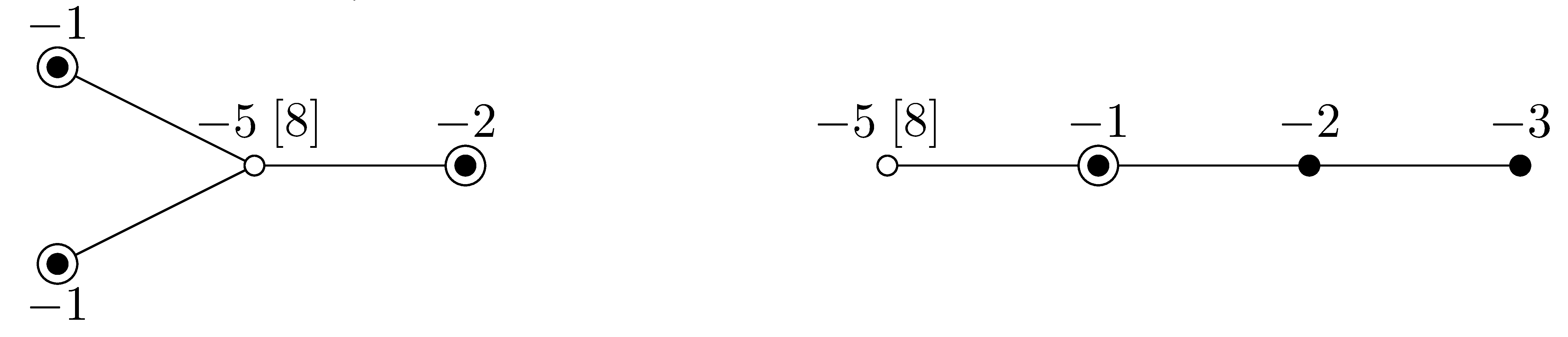
\( x^5+z^{15}+y^7z+txy^6=0 \).
Left: \( t\neq 0 \). Right: \( t=0 \).
Many explicit examples are described in
[7].
Let us give just one. Consider the
family of surface singularities \( (X_t,0)\subset (\mathbb{C}^3,0) \) with
equations \( x^5+z^{15}+y^7z+txy^6=0 \). It is the \( \mu \)-constant family
introduced by Briançon and Speder in
[e2].
It
has constant topological type, while the thick-thin decomposition
changes radically when \( t \) becomes 0. The two graphs of Figure 1
are the resolution graphs of \( \pi \) for \( t=0 \) and for
\( t \neq 0 \); the \( \mathcal L \)-nodes are the circled vertices, the subtrees
\( \Gamma_{\nu} \) corresponding to the components of the thick part have
black vertices, while the maximal subgraphs with white vertices
correspond to the components of the thin part. The negative number
weighting each vertex is the self-intersection of the corresponding
exceptional curve in \( \widetilde{X} \). The weight \( [8] \) means that
the corresponding exceptional curve has genus 8, while the others
have genus zero. For \( t \neq 0 \), \( (X_t,0) \) has three thick
components and a single thin one. For \( t =0 \), it has one component of
each type.
The second main result of [7], built on a refinement of the thick-thin decomposition, gives the complete inner Lipschitz classification of normal surface germs:
- the graph decomposition of \( X^{(\epsilon)} \) defined by the thick-thin decomposition;
- in the notation of Theorem 2.2, for each thin zone \( Z_j^{(\epsilon)} \), the homotopy class of the foliation by fibers of the fibration \( \zeta_j^{(\epsilon)}: Z_j^{(\epsilon)}\to S^1 \), and for each Seifert piece \( S_{\nu}^{(\epsilon)} \) of \( Z_j^{(\epsilon)} \), a rational number \( q_{\nu} \geq q_j \) with \( q_\nu=1 \) such that the fibers of the restriction \( \zeta_j^{(\epsilon)} \) to \( S_{\nu}^{(\epsilon)} \) have diameter of order \( \epsilon^{q_{\nu}} \).
The higher-dimensional case remains up to now almost unexplored.
3. Outer Lipschitz geometry
As already mentioned, the complete Lipschitz classification of complex curve germs for the outer metric was established by Frédéric Pham and Bernard Teissier in [e1] using the concept of Lipschitz saturations. In fact, any curve germ \( (X,0)\subset (\mathbb{C}^N,0) \) is bi-Lipschitz equivalent to its image \( (\ell(C), 0) \) by a generic linear plane projection \( \ell : \mathbb{C}^n \to \mathbb{C}^2 \). Therefore, it is sufficient to classify plane curve germs. The main result of [e1] says that the outer Lipschitz type of a complex curve germ \( (C,0) \subset (\mathbb{C}^2,0) \) determines and is determined by its embedded topological type, i.e., by the homeomorphism class of the pair \( (S^3_{\epsilon}, C^{(\epsilon)}) \). This result was revisited and completed by Walter and Anne with a geometric viewpoint:
- \( (C_1,0) \) and \( (C_2,0) \) have same Lipschitz
geometry, i.e., there is a homeomorphism of germs
\[\phi: (C_1,0)\to (C_2,0)\]
which is bi-Lipschitz for the outer metric;
- there is a homeomorphism of germs \( \phi: (C_1,0)\to (C_2,0) \), holomorphic except at 0, which is bi-Lipschitz for the outer metric;
- \( (C_1,0) \) and \( (C_2,0) \) have the same embedded topology, i.e., there is a homeomorphism of germs \( h: (\mathbb{C}^2,0) \to (\mathbb{C}^2,0) \) such that \( h(C_1)=C_2 \);
- there is a bi-Lipschitz homeomorphism of germs \( h: (\mathbb{C}^2,0) \to (\mathbb{C}^2,0) \) with \( h(C_1)=C_2 \).
The equivalence of (ii) and (iii) is the result of Pham and Teissier. The equivalence of (i), (iii) and (iv) is the new contribution. The proof of \( \text{(ii)} \Rightarrow \text{(iii)} \) based on what we call a bubble trick argument, which can be considered as a prototype for exploring Lipschitz geometry of singular spaces in various settings. An extended version of the proof is given in [e20]. The first occurence of a bubble trick argument we found in the litterature is in the paper of Jean-Pierre Henry and Adam Parusiński [e11]. This important tool is also used in recent works such has the construction of the moderately discontinuous homology by Javier Fernández de Bobadilla, Sonja Heinze, Maria Pe Pereira and José Edson Sampaio in [e18].
The question of the outer Lipschitz classification of higher-dimensional germs is still open. Actually, a very small amount of analytic invariants are determined by the topological type of an analytic germ (even if one considers the embedded topological type), and a first natural question to ask is whether the Lipschitz classification is sufficiently rigid to catch analytic invariants:
Which analytical invariants are in fact Lipschitz invariants?
During the last decade, it was shown that a large amount of analytic invariants are determined by the outer Lipschitz geometry in the case of a surface germ. The main result of [8] is the pioneering result in this direction. It shows that the outer Lipschitz class contains a lot of information on the singularity and confirms that outer Lipschitz geometry of singularities is a very promising area to explore. It can be seen as a first keystone to a complete classification of the outer Lipschitz geometry of complex surfaces. The higher-dimensional setting remains almost unexplored.
- the decorated resolution graph of the minimal good resolution of \( (X,0) \) which resolves the basepoints of a general linear system of hyperplane sections, i.e., the minimal good resolution which factors through the blow-up of the maximal ideal;
- the multiplicity of \( (X,0) \);
- the maximal ideal cycle in its resolution;
- for a generic hyperplane \( H \), the outer Lipschitz geometry of the curve \( (X\cap H,0) \);
- the decorated resolution graph of the minimal good resolution of \( (X,0) \) which resolves the basepoints of the family of polar curves of plane projections, i.e., the minimal good resolution which factors through the Nash modification;
- the topology of the discriminant curve of a generic plane projection;
- the outer Lipschitz geometry of the polar curve of a generic plane projection.
“Decorated resolution graph” means the resolution graph decorated with arrows corresponding to the components of the strict transform of the resolved curve.
The proof of this result is based on a sophisticated version of the bubble trick which leads to the graph decomposition of the link \( X^{(\epsilon)} \) described by the resolution graph of point (i).
The Lipschitz invariance of the multiplicity (point (ii) in the above theorem) was then extended beyond the normal case by Alexandre Fernandes and José Edson Sampaio ([e15]) for a hypersurface in \( \mathbb{C}^3 \) and by Javier Fernández de Bobadilla, Alexandre Fernandes and José Edson Sampaio ([e17]) for the general surface case. However it is now known that the multiplicity is not a Lipschitz invariant in higher dimensions ([e19]).
4. Lipschitz normal embeddings
Another important contribution of Walter in the area of Lipschitz geometry of singularities is his series of works on Lipschitz normal embedding. A subset (or a germ) in \( \mathbb{R}^n \) is Lipschitz Normally Embedded (LNE for short) if the identity map is a bi-Lipschitz homeomorphism (local in case of a germ) between the inner and outer metrics. Of course, every compact smooth submanifold in \( \mathbb{R}^n \) is LNE. But this property turns out to be fairly rare among singular spaces, and the results obtained by Walter with his coauthors suggest that it plays an important (quasi unexplored) role in several areas of singularity theory such as resolution of singularities or the structure of arc and jet spaces.
The pioneering result on LNE is the following theorem due to Lev and Tadeusz Mostowski. Its original version is proved in the semialgebraic setting, but this result remains true with the same proof in the more general subanalytic category and even, in the o-minimal category. We state it here in the subanalytic setting.
The map \( p : X \rightarrow \widetilde{X} \) is called a normal embedding of \( X \).
As a consequence of this theorem, one obtains the following alternative definition of the notion of Lipschitz normal embedding. The proof was never written before. That is why we include it in this manuscript.
Proof. Assume there exist a subanalytic bi-Lipschitz homeomorphism \( f : (X,d_i) \to (X,d_o) \) and a real number \( K\geq 1 \) as in the statement. Let \( p : (X,d_i) \to ( \widetilde{X},d_i) \) be a normal embedding of \( X \) as in Theorem 4.1. We deduce that \( p \circ f^{-1} \) is bi-Lipschitz with respect to the outer metrics. Therefore \( p \circ f^{-1} \) is also bi-Lipschitz with respect to the inner metrics. This implies that \( \mathrm{Id}_X = f \circ f^{-1} = f \circ p^{-1} \circ p \circ f^{-1} \) is bi-Lipschitz from \( (X,d_i) \) to \( (X,d_o) \). ☐
Complex and real algebraic sets of \( \mathbb{C}^n \) or \( \mathbb{R}^n \) are subanalytic sets. By Theorem 4.1, they admit a global subanalytic Lipschitz normal embedding. Tadeusz Mostowski asked if there exists a complex algebraic Lipschitz normal embedding when \( X \) is a complex algebraic set, i.e., a (subanalytic) Lipschitz normal embedding for which the image set \( \tilde{X}\subset\mathbb{C}^n \) is a complex algebraic set.
The answer is positive in complex dimension 1: every complex algebraic curve admits a complex algebraic Lipschitz normal embedding. This follows from the fact that an irreducible germ of complex algebraic curve is subanalytically bi-Lipschitz homeomorphic with respect to the inner metric to the germ of \( \mathbb{C} \) at the origin (see for example Proposition 2.1 of [8]). Then a normal embedding can be constructed by using the so-called tent procedure introduced in [e9].
Walter, Lev and Alexandre Fernandes answered negatively to Mostowski’s question in higher dimension by proving the following result:
admits a complex algebraic normal embedding.
The proof of this result is based on a beautiful topological argument due to Walter that we reproduce here:
Proof. Assume there exists a complex algebraic Lipschitz normal embedding \( p : X \to\widetilde{X} \). By Theorem 1.3 of [2], the germ \( (X,0) \) is metrically conical for the inner metric by a subanalytic homeomorphism, and so is \( (\widetilde{X},0) \). Since \( (\widetilde{X},0) \) is LNE, it is then subanalytically metrically conical for the outer metric. By a result of Bernig and Lytchak (see Remark 2, Theorem 1.2 of [e12]), this implies that \( (\widetilde{X}, 0) \) is subanalytically bi-Lipschitz homeomorphic to its tangent cone \( C_0 \widetilde{X} \) at 0 for the outer metric, which is the complex cone over a projective algebraic curve \( C \). Since \( (X,0) \) has isolated singularity, then its link is a topological manifold, which implies that \( C \) is irreducible and locally irreducible. Now, if \( C \) had a singular point, this would contradict the fact that \( C_0 \widetilde{X} \) is LNE. Therefore, \( C_0\widetilde{X} \) is a complex algebraic cone over a smooth irreducible projective curve, thus its link is a \( S^1 \)-bundle. On the other hand, the link of \( X \) at 0 is a Seifert fibered manifold with \( b \) singular fibers of degree \( a/\gcd(a,b) \). This is a contradiction because the Seifert fibration of a Seifert fibered manifold (other than a lens space) is unique up to diffeomorphism. ☐
Another important contribution of Walter is a characterization of normal surface singularities which are LNE. In [e16], Lev proved with Rodrigo Mendes that a semialgebraic germ \( (X,0) \) is LNE if and only if if all pairs of real arcs \( p_1 \) and \( p_2 \) in \( (X,0) \) have equal inner and outer contacts. This criterion is difficult to use effectively in practice to prove LNE-ness of a germ since it requires to compute the inner and outer contact orders of an immense amount of pairs of arcs. Walter, with Anne and Helge Pedersen, established in [9] an analogous criterion for complex surface germs where the number of pairs of arcs to be tested is reduced drastically to just finitely many types of pairs.
This efficient LNE criterion led to the discovery of several nontrivial infinite family of LNE normal surface germs. For example:
Minimal singularities were introduced by Janos Kollár in [e5]. In dimension 2, they are rational surface singularities which play a major role in resolution theory (see [e7], [e10]).
Several other families were discovered later using the criterion of
[9],
for example among super-isolated
singularities
[e21].
But LNE-ness of complex surfaces
is far from being completely understood, and the higher-dimensional
case is still in its infancy.
5. Dissemination
In June 2018, Walter organized with Anne an international school on Lipschitz geometry of singularities in Cuernavaca, Mexico. About fifty PhD students and young researchers attended the event, and the theory and promising extensions were introduced a huge variety of viewpoints, by Walter himself and also Patrick Popescu-Pampu, Maria Aparecida Soares Ruas, Bernard Teissier, David Trotman, among others.
The lecture notes were completed and collected in a Lecture Notes in Mathematics volume [11], edited by Walter and Anne, which is the first introductory book on Lipschitz geometry of singularities, and which is now in the hands of many PhD students and young researchers. The volume also contains an english version of the historical paper of Pham and Teissier [e1], which was a preprint in French of the École Polytechnique during 50 years.
