Celebratio Mathematica

The group \( \operatorname{SL}_2(\mathbb R) \) acts on the up­per half-plane \( \mathfrak H \) by frac­tion­al lin­ear trans­form­a­tions. A clas­sic­al mod­u­lar form is a holo­morph­ic func­tion on \( \mathfrak H \) with sym­met­ries with re­spect to a con­gru­ence sub­group \( \Gamma \) of \( \operatorname{SL}_2(\mathbb Z) \). It is called a cusp form if it van­ishes at the cusps of \( \Gamma \). A mod­u­lar form has a Four­i­er ex­pan­sion. His­tor­ic­ally, the arith­met­ic of mod­u­lar forms is un­der­stood by way of study­ing their Four­i­er coef­fi­cients. The twen­ti­eth cen­tury wit­nessed fant­ast­ic ad­vance­ments in mod­u­lar forms, from the­ory to ap­plic­a­tions. Lis­ted be­low are some land­mark break­throughs rel­ev­ant to the theme of this art­icle.

1. In the 1930s Hecke in­tro­duced the Hecke op­er­at­ors \( T_p \) for primes \( p \) act­ing on mod­u­lar forms, thereby re­du­cing the study of mod­u­lar forms to com­mon ei­gen­forms of \( T_p \) (see [e5], Num­bers 39, 40).
2. Weil’s con­verse the­or­em [e9] of 1967 provides an ana­lyt­ic cri­terion for a holo­morph­ic func­tion on \( \mathfrak H \) defined by giv­en Four­i­er coef­fi­cients to be a mod­u­lar form for \( \Gamma_0(N) \). This ori­gin­ates from Hecke’s con­verse the­or­em for mod­u­lar forms for \( \operatorname{SL}_2(\mathbb Z) \), namely the case \( N=1 \) [e1].
3. Atkin and Lehner’s new­form the­ory [e10] of 1970 fur­ther re­duces the study of com­mon Hecke ei­gen­forms for con­gru­ence sub­groups of type \( \Gamma_0(N) \) to new­forms.

The con­verse the­or­em (2) and the new­form the­ory (3) were ex­ten­ded to all clas­sic­al mod­u­lar forms in the 1970s by Miyake [e12] and Li [e16].

An­drew Ogg made im­port­ant con­tri­bu­tions to clas­sic­al mod­u­lar forms in the 1960s and the 1970s. His 1969 Ben­jamin notes Mod­u­lar Forms and Di­rich­let Series [1] elab­or­ated the con­verse the­or­em by Hecke and Weil, among oth­er things. It was a pop­u­lar book in mod­u­lar forms for a long time.

To ex­plain his con­tri­bu­tion to the new­form the­ory, let \[ f(\tau) = \sum_{n\ge 1} a_n e^{2\pi i n\tau} \] be a cuspid­al new­form of weight \( k \) level \( N \) and char­ac­ter \( \chi \), nor­mal­ized with \( a_1=1 \). Then \( f \) is an ei­gen­func­tion of the Hecke op­er­at­or \( T_p \) with ei­gen­value \( a_p \) for primes \( p\, \nmid\, N \), and the Four­i­er coef­fi­cients \( a_n \) are de­term­ined by \( a_p \) for all primes \( p \) in the fol­low­ing way, ex­pressed in terms of the L-func­tion at­tached to \( f \): \begin{align*} L(f,s) &=\sum_{n\ge 1} a_n n^{-s}\\ &= \prod_{p\,|\,N}\,\frac{1}{1-a_p p^{-s}} ~\prod_{p\, \nmid\, N}\,\frac{1}{1 - a_pp^{-s} + \chi(p)p^{k-1-2s}}. \end{align*}

For primes \( p \,\nmid\, N \), the Ramanu­jan con­jec­ture, proved by De­ligne [e13], [e14] for weight \( k > 2 \), by Eichler and Shimura [e2], [e4] for \( k=2 \), and by De­ligne and Serre [e15] for \( k=1 \), as­serts that \[ |a_p| \le 2p^{(k-1)/2}. \] The size of \( a_p \) for \( p\,|\,N \), as de­scribed be­low, was proved in [e16] us­ing a the­or­em of Ogg in [3]:

\( |a_p| = p^{(k-1)/2} \) if \( \chi \) is not a char­ac­ter mod \( N/p \); when \( \chi \) is a char­ac­ter mod \( N/p \), then \( a_p^2 = \chi(p)p^{k-2} \) if \( p\parallel N \), and \( a_p=0 \) oth­er­wise.

Ogg also stud­ied con­vo­lu­tion of L-series at­tached to cusp forms. Giv­en two cusp forms \( f \) and \( g \) of weight \( k \) and level \( N \) with Four­i­er coef­fi­cients \( \{a_n\} \) and \( \{b_n\} \) re­spect­ively, Rankin in­tro­duced the con­vo­luted L-series \[ L_{f,g}(s) = \prod_{p\,\nmid\, N}\,\frac{1}{1-p^{-2s}} \,\sum_{n \ge 1} \,a_n \overline{b_n} n^{-(s-k+1)} \] defined for \( \Re s \) large. When \( N=1 \), he showed that it had an ana­lyt­ic con­tinu­ation to the whole com­plex plane and ob­tained a func­tion­al equa­tion re­lat­ing the val­ues at \( s \) and \( 1-s \). Ogg [2] ex­ten­ded this to square-free \( N \) by sup­ple­ment­ing the miss­ing Euler factors at primes di­vid­ing \( N \).

The case for any pair of new­forms was done in late 1970s in [e16], [e19]. Lang­lands re­in­ter­preted the L-func­tions at­tached to cuspid­al new­forms as L-func­tions at­tached to cuspid­al auto­morph­ic rep­res­ent­a­tions of \( \operatorname{GL}_2 \) over \( \mathbb Q \). In the con­text of rep­res­ent­a­tion the­ory, the above res­ult can be re­ph­rased as de­term­in­ing the loc­al L- and \( \epsilon \)-factors of \( \pi_1 \times \pi_2 \) for two cuspid­al auto­morph­ic rep­res­ent­a­tions \( \pi_1 \) and \( \pi_2 \) of \( \operatorname{GL}_2 \) over \( \mathbb Q \) so that, when mul­ti­plied to­geth­er, they give rise to a glob­al func­tion­al equa­tion for the L-func­tion \( L(\pi_1 {\times} \pi_2, s) \) un­der \( s \to 1-s \).

We have seen that a new­form is a com­mon ei­gen­func­tion of the Hecke op­er­at­ors and is de­term­ined by the ei­gen­val­ues of the Hecke op­er­at­ors. Thus it is nat­ur­al to ask, giv­en a con­gru­ence sub­group \( \Gamma \) of \( \operatorname{SL}_2(\mathbb R) \), how to com­pute the traces of Hecke op­er­at­ors on the space of mod­u­lar forms for \( \Gamma \) with a giv­en weight. Since the space of mod­u­lar forms for \( \Gamma \) de­com­poses as the dir­ect sum of the space of Ei­s­en­stein series and the space of cusp forms, and the former is well un­der­stood, we are in­ter­ested in ex­pli­cit trace for­mu­lae of Hecke op­er­at­ors on the space \( S_{k+2}(\Gamma) \) of cusp forms of weight \( k+2\ge 2 \) for \( \Gamma \). When \( k=0 \), the cusp forms of weight 2 are in one-to-one cor­res­pond­ence with holo­morph­ic dif­fer­en­tials on the com­pac­ti­fied mod­u­lar curve \( X_\Gamma= \Gamma \backslash \mathfrak H^* \), where \( \mathfrak H^* \) is \( \mathfrak H \) for \( \Gamma \) cocom­pact, and it is \( \mathfrak H \cup \{\text{cusps}\} \) for \( \Gamma \) non-cocom­pact; hence the di­men­sion of the space \( S_2(\Gamma) \) is the genus of \( X_\Gamma \). In par­tic­u­lar, \( S_2(\Gamma) \) is trivi­al if \( X_\Gamma \) has genus 0. Fur­ther­more, we shall as­sume \( k \) even if \( -\operatorname{Id} \in \Gamma \) be­cause in this case the space is trivi­al for \( k \) odd.

This was done by Ahl­gren [e27] for \( \Gamma_0(4) \); Ahl­gren and Ono [e26] for \( \Gamma_0(8) \); Frechette, Ono and Papan­ikolas [e28] for new­forms of \( \Gamma_0(8) \); Fuse­li­er [e31], [e35] for \( \operatorname{SL}_2(\mathbb Z) \); and Len­non [e33], [e32] for \( \Gamma_0(3) \) and \( \Gamma_0(9) \). They all fol­lowed Ihara’s ap­proach in [e8], com­bin­ing count­ing el­lipt­ic curves over fi­nite fields with the Sel­berg trace for­mula. In [e38] Ono and Saad did it for \( \Gamma_0(2) \) and \( \Gamma_0(4) \), fol­low­ing Za­gi­er’s work [e25] for \( \operatorname{SL}_2(\mathbb Z) \). Their meth­od uses the Rankin–Co­hen brack­ets of Za­gi­er’s mock mod­u­lar form.

All the groups men­tioned above have genus 0 and are non-cocom­pact. When \( \Gamma \) is cocom­pact, the mod­u­lar curve \( X_\Gamma \) is called a Shimura curve. It has no cusps. In this case we identi­fy the space of mod­u­lar forms with cusp forms of \( \Gamma \) by ab­use of lan­guage. Ogg was in­ter­ested in Shimura curves \( X_\Gamma \) and mod­u­lar forms for \( \Gamma \) in the 1980s. See [4], [5]. While Hecke op­er­at­ors on forms for a cocom­pact \( \Gamma \) is defined the same way as \( \Gamma \) non-cocom­pact, however, due to the lack of cusps, there is no a pri­ori choice of a point on the Shimura curve \( X_\Gamma \) to play the role of the cusp at \( \infty \) for non-cocom­pact groups to fa­cil­it­ate the study of the Hecke op­er­at­ors. This has been a ma­jor obstacle in study­ing the arith­met­ic of mod­u­lar forms on Shimura curves. Yang’s pa­per [e34] well il­lus­trates this point.

In­spired by Long, Li and Tu [e37] and by Scholl [e22], in a re­cent joint work with Hoff­man, Long and Tu [e39], we ob­tained ex­pli­cit trace for­mu­lae of Hecke op­er­at­ors on \( S_{k+2}(\Gamma) \) in terms of hy­per­geo­met­ric char­ac­ter sums for cer­tain arith­met­ic tri­angle groups \( \Gamma \). Our geo­met­ric ap­proach gives a uni­fied treat­ment for \( \Gamma \) el­lipt­ic mod­u­lar (the non-cocom­pact case), in­clud­ing afore­men­tioned groups, and \( \Gamma \) arising from the in­def­in­ite qua­ternion al­gebra \( B_6 = \bigl(\frac{-1, 3}{\mathbb{Q}}\bigr) \) over \( \mathbb{Q} \) with dis­crim­in­ant 6 (the cocom­pact case). The same meth­od can also be ap­plied to ob­tain ei­gen­val­ues of the Hecke op­er­at­ors as well.

Let \( \Gamma \) be a con­gru­ence sub­group com­men­sur­able with \( \operatorname{SL}_2(\mathbb Z) \) (hence non-cocom­pact) or the norm 1 group \( \mathcal O^1 \) of a max­im­al or­der \( \mathcal O \) of an in­def­in­ite non­split qua­ternion al­gebra \( B \) over \( \mathbb{Q} \) (hence cocom­pact). As­sume the com­pac­ti­fied mod­u­lar curve \( X_\Gamma \) has Shimura ca­non­ic­al mod­el defined over \( \mathbb{Q} \).

The first geo­met­ric in­ter­pret­a­tion of the Hecke op­er­at­ors was the cel­eb­rated Eichler–Shimura con­gru­ence re­la­tion in­tro­duced by Eichler [e2] and gen­er­al­ized by Shimura [e4] for Hecke op­er­at­ors act­ing on weight-2 cusp forms for el­lipt­ic mod­u­lar groups. This was ex­ten­ded to qua­ternion­ic groups by Kuga and Shimura [e7]. For forms of weight \( k+2 \ge 3 \), us­ing the mod­uli in­ter­pret­a­tion of \( X_\Gamma \), De­ligne [e13] for \( \Gamma \) non-cocom­pact and Ohta [e20] for \( \Gamma \) cocom­pact con­struc­ted, for each prime \( \ell \), an auto­morph­ic \( \ell \)-ad­ic sheaf \( V^k(\Gamma)_\ell \) on \( X_\Gamma \otimes \overline {\mathbb Q} \) which provided the fol­low­ing geo­met­ric in­ter­pret­a­tion of the Hecke traces.

Com­bined with the Grothen­dieck–Lef­schetz fixed point for­mula, we ob­tain a geo­met­ric in­ter­pret­a­tion of the Hecke trace in terms of the sum of Frobeni­us traces: \begin{eqnarray} -{\operatorname{Tr}} (T_p\mid S_{k+2} (\Gamma)) = \sum_{\lambda \in X_{\Gamma}(\mathbb F_p)} {\operatorname{Tr}}({\operatorname{Frob}}_\lambda \mid (V^{k} (\Gamma)_{\ell})_{\bar{\lambda}} ). \end{eqnarray}

Here \[ {\operatorname{Tr}}({\operatorname{Frob}}_\lambda \mid (V^{k} (\Gamma)_{\ell})_{\bar{\lambda}} )= {\operatorname{Tr}}({\operatorname{Frob}}_\mathfrak P \mid (V^{k} (\Gamma)_{\ell})_{\bar{\lambda^{\prime}}} ) \] for any al­geb­ra­ic point \( \lambda^{\prime} \) on \( X_\Gamma \) which re­duces to \( \lambda \) mod­ulo a de­gree-1 prime \( \mathfrak P \) above \( p \).

Equa­tion (1) would give an ex­pli­cit Hecke trace for­mula if one could com­pute the Frobeni­us traces on stalks of the auto­morph­ic sheaf. We show that this can be car­ried out when the group \( \Gamma \) is an arith­met­ic tri­angle group of type (a) or (b) as spe­cified in Sec­tion 2.1. More pre­cisely, we prove that, for such a \( \Gamma \), the auto­morph­ic sheaf with min­im­al \( k \), namely \( V^1(\Gamma)_\ell \) for \( \Gamma \) of type (a) and \( V^2(\Gamma)_\ell \) for \( \Gamma \) of type (b), up to twist by a de­gree-1 sheaf, is iso­morph­ic to the hy­per­geo­met­ric sheaf at­tached to the hy­per­geo­met­ric datum \( \operatorname{HD}(\Gamma) \) in­tro­duced by Katz in [e24] [e30] and fur­ther ex­ten­ded by Beuk­ers, Co­hen and Mel­lit in [e36] for which the Galois ac­tion on a stalk has Frobeni­us traces ex­pli­citly ex­pressed by hy­per­geo­met­ric char­ac­ter sums. Since, as ex­plained in Sec­tion 3.1, for the groups we con­sider the Frobeni­us traces on sheaves with lar­ger \( k \) are sym­met­ric powers of those with min­im­al \( k \), we ob­tain de­sired Hecke traces for all \( k \ge 1 \).

Our uni­fied ap­proach has the fol­low­ing two mer­its.

I. Sup­pose the space \( S_{k+2}(\Gamma) \) has di­men­sion \( m \). Us­ing the same meth­od, we can com­pute the traces of \( (\operatorname{Frob}_{p})^r \) for \( 1 \le r \le m \), which in turn give rise to the ei­gen­val­ues of \( T_p \) on \( S_{k+2}(\Gamma) \). This is es­pe­cially use­ful when we ex­plore Hecke ei­gen­val­ues for mod­u­lar forms on Shimura curves.

II. Let \( \Gamma^{\prime} \) be a con­gru­ence sub­group of \( \Gamma \), where \( \Gamma \) is an arith­met­ic tri­angle group of type (a) or (b) while \( \Gamma^{\prime} \) is not. As­sume that the curve \( X_{\Gamma^{\prime}} \) is defined over \( \mathbb{Q} \) and there is an ex­pli­cit \( \mathbb{Q} \)-ra­tion­al cov­er­ing map \( \pi: X_{\Gamma^{\prime}} \to X_{\Gamma} \). Then the auto­morph­ic sheaves on \( X_{\Gamma^{\prime}} \) are the pull-backs of those on \( X_{\Gamma} \) via \( \pi^* \). By pulling back the hy­per­geo­met­ric sheaf on \( X_\Gamma \) via \( \pi^* \) we can ex­press the Hecke traces on \( S_{k+2}(\Gamma^{\prime}) \) ex­pli­citly in terms of the hy­per­geo­met­ric char­ac­ter sums at­tached to \( \operatorname{HD}(\Gamma) \).

This pa­per is or­gan­ized as fol­lows. After de­scrib­ing in Sec­tion 2.1 the arith­met­ic tri­angle sub­groups \( \Gamma \) of types (a) and (b) to be con­sidered in this pa­per, in Sec­tion 2.2 the ex­pli­cit trace for­mula for the Hecke op­er­at­or \( T_p \) on \( S_{k+2}(\Gamma) \) is stated in The­or­em 2 for \( \Gamma \) of type (a) and in The­or­em 3 of type (b). Two ex­amples for the cocom­pact group \( \Gamma=(2,4,6) \) of type (b) are il­lus­trated in Sec­tion 2.3. The first is the trace for­mula for the one-di­men­sion­al \( S_8(2,4,6) \), in this case the trace of \( T_p \) is also the ei­gen­value of \( T_p \). The second is the two-di­men­sion­al \( S_{24}(2,4,6) \). We demon­strate that by ap­ply­ing the same meth­od to com­pute the traces of \( \operatorname{Frob}_p \) and \( (\operatorname{Frob}_{p})^2 \), we ob­tain the two ei­gen­val­ues of \( T_p \). As an ap­plic­a­tion, The­or­em 4 in Sec­tion 2.4 gives the trace of \( T_p \) on \( S_{k+2}(2,6,6) \) ex­pressed in terms of hy­per­geo­met­ric char­ac­ter sums at­tached to the datum for \( (2,4,6) \). Ob­serve that \( (2,6,6) \) is not of type (a) or (b). The trace for­mula is ob­tained by pulling back the hy­per­geo­met­ric sheaf on \( X_{(2,4,6)} \) along the ex­pli­cit 2-fold pro­jec­tion \( \pi_2: X_{(2,6,6)} \to X_{(2,4,6)} \) defined over \( \mathbb{Q} \). The auto­morph­ic sheaves \( V^k(\Gamma) \) and hy­per­geo­met­ric sheaves \( \mathcal H(\operatorname{HD}(\Gamma)) \) on \( X_\Gamma \) as well as their key prop­er­ties are re­called in Sec­tion 3.1 and Sec­tion 3.2, re­spect­ively, each hav­ing a com­plex part af­ford­ing the ac­tion of \( \Gamma \) and an \( \ell \)-ad­ic coun­ter­part for each prime \( \ell \) af­ford­ing Galois ac­tions. In geo­met­ric lan­guage, these two parts can be com­bined and re­in­ter­preted as a sheaf on \( X_\Gamma \) of its étale fun­da­ment­al group. A sketch of the proof of our main res­ults, The­or­ems 2 and 3, is giv­en in Sec­tion 4. We use Katz’s ri­gid­ity the­or­em (The­or­em 7) and our com­par­is­on the­or­em (The­or­em 8) to prove that \( V^1(\Gamma) \simeq \mathcal H(\operatorname{HD}(\Gamma)) \) for \( \Gamma \) of type (a) and \( V^2(\Gamma) \) is iso­morph­ic to the twist of \( \mathcal H(\operatorname{HD}(\Gamma)) \) by an ex­pli­cit de­gree-1 sheaf for \( \Gamma \) of type (b). This gives rise to the con­tri­bu­tions of \( \operatorname{Frob}_\lambda \) at nonsin­gu­lar \( \lambda \in X_\Gamma(\mathbb F_p) \) in (1), which cor­res­pond to \( \lambda \in \mathbb F_p^\times, \lambda \ne 1 \) in the trace for­mu­las stated in The­or­ems 2 and 3. Sin­gu­lar points of \( X_\Gamma(\mathbb F_p) \) arise from the cusps and el­lipt­ic points of \( X_\Gamma \). The con­tri­bu­tion at a cusp is 1 for \( k \) even; for \( k \) odd, it is \( \pm 1 \) or 0, de­pend­ing on the type of re­duc­tion at \( p \) of the de­gen­er­ate el­lipt­ic curve rep­res­ent­ing the cusp. Each el­lipt­ic point \( \lambda \) of \( X_\Gamma \) is a CM point. The con­tri­bu­tion at \( \lambda \) de­pends on \( k \), the or­der of the point and the be­ha­vi­or of \( p \) in the CM field. The con­tri­bu­tions at sin­gu­lar points are com­puted sep­ar­ately, and the cel­eb­rated Néron–Ogg–Sha­far­ev­ich cri­terion is used.

Let \( e_1, e_2, e_3 \) be ele­ments in \( \mathbb Z_{ > 0} \cup\{\infty\} \). Defined in terms of gen­er­at­ors and re­la­tions, an arith­met­ic tri­angle group \[ (e_1, e_2, e_3) := \langle g_1, g_2, g_3~|~g_1^{e_1} = g_2^{e_2} = g_3^{e_3} = g_1g_2g_3= \operatorname{Id} \rangle \] can be real­ized as a dis­crete sub­group \( \Gamma \) of \( \operatorname{PSL}_2(\mathbb R) \) act­ing on \( \mathfrak H \). A fun­da­ment­al do­main of \( \Gamma \) is a tri­angle with the three ver­tices \( v_1, v_2, v_3 \) sta­bil­ized by (a con­jug­ate of) \( g_1, g_2, g_3 \), re­spect­ively. Here \( v_i \) is a cusp of \( \Gamma \) if \( e_i = \infty \); if \( e_i \) is a pos­it­ive in­teger, then \( v_i \) is an el­lipt­ic point of or­der \( e_i \). These groups are clas­si­fied by Takeu­chi [e17], [e18]. In or­der that the com­pac­ti­fied mod­u­lar curve \( X_\Gamma \) af­ford a hy­per­geo­met­ric sheaf over \( \mathbb{Q} \), it must be of genus zero and its Shimura ca­non­ic­al mod­el must be defined over \( \mathbb{Q} \) with the three ver­tices of \( X_\Gamma \) of or­ders \( e_1, e_2, e_3 \) be­ing \( \mathbb{Q} \)-ra­tion­al. As ex­plained in ([e39], Sec­tion 3), the con­cerns on the re­quired prop­er­ties of the hy­per­geo­met­ric sheaves on \( X_\Gamma \) led us to the sev­en sub­groups, \( \Gamma = (e_1, e_2, e_3) \) lis­ted be­low; those of type (a) are iso­morph­ic to a sub­group of \( \operatorname{SL}_2(\mathbb Z) \) not con­tain­ing \( -\operatorname{Id} \), while those of type (b) are iso­morph­ic to a sub­group of \( \operatorname{SL}_2(\mathbb R) \) mod­ulo \( \pm \operatorname{Id}{:} \)

1. \( (3, \infty, \infty) \simeq \Gamma_1(3) \),
   \( (\infty, \infty, \infty) \simeq \Gamma_1(4) \);
2. \( (2, \infty, \infty) \simeq \Gamma_0(2)/\{\pm \operatorname{Id}\} \),
   \( (2,3, \infty) \simeq \operatorname{PSL}_2(\mathbb Z) \),
   \( (2,4, \infty) \simeq \langle \Gamma_0(2), w_2\rangle/\{\pm \operatorname{Id}\}=\Gamma_0(2)^+/\{\pm \operatorname{Id}\} \),
   \( (2,6,\infty) \simeq \langle \Gamma_0(3), w_3 \rangle/\{\pm \operatorname{Id}\}=\Gamma_0(3)^+/\{\pm \operatorname{Id}\} \),
   \( (2,4,6) = \langle \mathcal O_{B_6}^1, w_2, w_3, w_6\rangle/\{\pm \operatorname{Id}\} \).

Here \( w_2, w_3, w_6 \) are the Atkin–Lehner in­vol­u­tions. They are well known for con­gru­ence sub­groups of \( \operatorname{SL}_2(\mathbb Z) \). We ex­plain those for the qua­ternion al­gebra \( B_6 \). A max­im­al or­der of \( B_6 \), which is unique up to con­jug­a­tion, is \[ \mathcal O_{B_6} = \mathbb Z + \mathbb ZI + \mathbb ZJ + \mathbb Z \,\frac{1+I+J+IJ}{2}, \] where \( I^2=-1 \),  \( J^2=3 \),  \( IJ=-JI \). The Atkin–Lehner in­vol­u­tions \( w_6, w_2, w_3 \) are defined as the ele­ments \( 3I+IJ \),  \( 1+I \),  \( (3+3I+J+IJ)/2 \) of \( \mathcal O_{B_6} \), re­spect­ively, nor­mal­ized by di­vid­ing by the pos­it­ive square root of the re­spect­ive re­duced norm 6, 2, 3. They act on the curve \( X_{(2,4,6)} \) and sta­bil­ize the el­lipt­ic points of or­ders \( 2,4,6 \), re­spect­ively.

A hy­per­geo­met­ric datum is a set \( \operatorname{HD}=\{\alpha, \beta\} \), where \( \alpha=\{a_1,\dots, a_n\} \) and \( \beta=\{b_1=1, b_2,\dots, b_n\} \) are multis­ets with \( a_i, b_j \in \mathbb{Q}^\times \). It is prim­it­ive if \( a_i -b_j \notin \mathbb Z \) for \( 1 \le i, j \le n \). We as­so­ci­ate a prim­it­ive hy­per­geo­met­ric datum \( \operatorname{HD}(\Gamma) = \{\alpha(\Gamma), \beta(\Gamma)\} \) to each of the above sev­en sub­groups \( \Gamma \), as shown in Table 1. \begin{gather*} \begin{array}{|c|c|c|c|c|c|c|c|c|c|c|c|c|c|} \hline \Gamma=(e_1,e_2,e_3)&(3, \infty, \infty) & (\infty, \infty, \infty) & (2,\infty,\infty)&(2,3,\infty)&(2,4,\infty)&(2,6,\infty)&(2,4,6)\\ \hline \alpha(\Gamma) & \bigl\{\frac13, \frac23\bigr\} & \bigl\{\frac12, \frac12\bigr\} & \bigl\{\frac12,\frac12,\frac12\bigr\} &\bigl\{\frac12,\frac16,\frac56\bigr\}&\bigl\{\frac12,\frac14,\frac34\bigr\}&\bigl\{\frac12,\frac13,\frac23\bigr\}&\bigl\{\frac12,\frac14,\frac34\bigr\}\\ \beta(\Gamma)& \{1,1\} & \{1,1\} & \{1,1,1\}&\{1,1,1\}&\{1,1,1\}&\{1,1,1\}& \bigl\{1,\frac56,\frac76\bigr\}\\ \hline \end{array} \\ \textbf{Table 1.}\,\text{The hypergeometric datum } \operatorname{HD}(\Gamma) \text{ attached to } \Gamma. \end{gather*}

When the sets \( \alpha, \beta \) in a prim­it­ive hy­per­geo­met­ric datum \( \operatorname{HD}=\{\alpha, \beta\} \) are defined over \( \mathbb{Q} \), for each prime \( p \) and \( \lambda \in \mathbb F_p^\times \), Beuk­ers, Co­hen and Mel­lit defined in [e36] the hy­per­geo­met­ric char­ac­ter sum \( H_p(\operatorname{HD}, \lambda) \). The de­tailed defin­i­tion is a bit long and will be omit­ted. To give a fla­vor, sup­pose \( \alpha=\{a_1,\dots, a_n\} \), \( \beta=\{b_1=1, b_2,\dots, b_n\} \). Con­sider primes \( p \equiv 1 \pmod M \), where \( M = \operatorname{lcd}(\operatorname{HD}) \) is the least com­mon de­nom­in­at­or of all \( a_i \) and \( b_j \). Let \( \lambda \in \mathbb F_p^\times \). Then \( H_p(\operatorname{HD}, \lambda) \) can be ex­pressed in terms of Gauss sums as fol­lows: \[ H_p(\operatorname{HD}(\Gamma), \lambda) = \,\frac{1}{1-p}\sum_{s=0}^{p-2}\omega^s((-1)^n\lambda)\prod_{j=1}^n\,\frac{g(\omega^{(p-1)a_j+s})g(\bar{\omega}^{(p-1)b_j+s})}{g(\omega^{(p-1)a_j})g(\bar{\omega}^{(p-1)b_j})}. \] In the above, \( \omega \) is a char­ac­ter of \( \mathbb F_p^\times \) of or­der \( p-1 \), and \( g(\omega^j) \) is the Gauss sum at­tached to the char­ac­ter \( \omega^j \) and a fixed non­trivi­al ad­dit­ive char­ac­ter of \( \mathbb F_p \). The res­ult­ing ex­pres­sion is in­de­pend­ent of the choice of the ad­dit­ive char­ac­ter and \( \omega \) for our \( \alpha, \beta \) since they are defined over \( \mathbb{Q} \). Note that when char­ac­ters \( \omega^{(p-1)b_j+s} \) and \( \omega^{(p-1)b_j} \) are non­trivi­al, we have \[ \omega^s(-1)\,\frac{g(\omega^{(p-1)a_j+s})g(\bar{\omega}^{(p-1)b_j+s})}{g(\omega^{(p-1)a_j})g(\bar{\omega}^{(p-1)b_j})} = \frac{g(\omega^{(p-1)a_j+s})/g(\omega^{(p-1)a_j})}{g(\omega^{(p-1)b_j+s})/g(\omega^{(p-1)b_j})} \] by a Gauss sum iden­tity. There­fore \( H_p(\operatorname{HD},\lambda) \) is re­garded as a fi­nite field ana­log of the com­plex-val­ued clas­sic­al hy­per­geo­met­ric func­tion \( _nF_{n-1}(\alpha, \beta; \lambda) \) defined by \[_nF_{n-1}(\alpha, \beta; \lambda) = \sum_{s=0}^{\infty} \prod_{j=1}^n \,\frac{\Gamma(a_j+s)/\Gamma(a_j)}{\Gamma(b_j+s)/\Gamma(b_j)} \lambda^s \] in terms of the usu­al \( \Gamma \)-func­tion for \( \lambda \in {\mathbb C} \) such that the series con­verges.

We shall ex­press Tr\( (T_p, S_{k+2}(\Gamma)) \) in terms of these hy­per­geo­met­ric char­ac­ter sums ac­cord­ing to the type of \( \Gamma \).

De­note by \( N_\Gamma = 3 \) (resp. 4) the level of the group \( (3, \infty, \infty)=\Gamma_1(3) \) (resp. \( (\infty, \infty, \infty) = \Gamma_1(4) \)). Ob­serve that \( {\operatorname{Tr}}(T_p, S_{k+2}(\Gamma))=0 \) when \( p \equiv -1 \mod N_\Gamma \) and \( k \) is odd.

To state our res­ults for groups of type (b), for in­tegers \( m \ge 1 \), let \( F_m(S, T) \) be the de­gree-\( m \) poly­no­mi­al in \( S \) and \( T \) defined by the re­curs­ive re­la­tion \begin{align} & F_{m+1}(S, T) = (S-T)F_m(S, T) - T^2F_{m-1}(S, T),\notag\\ \label{F_m} & F_0(S, T) = 1, \quad F_1(S, T)=S. \end{align}

In fact, we may choose \( \alpha_{N(z),p} \) to be the Jac­obi sum \( J_\omega\bigl(\frac13,\frac13\bigr) \) (resp. \( J_\omega\bigl(\frac14,\frac14\bigr) \)) if \( N(z) \in \{3, 6\} \) (resp. \( N(z) = 4 \)). Here \( \omega \) is any gen­er­at­or of the group of char­ac­ters of \( \mathbb F_p^\times \). We re­mark that a Jac­obi sum \( J_\omega(a,b) \) is it­self a hy­per­geo­met­ric char­ac­ter sum.

To ex­hib­it con­crete ex­amples, con­sider mod­u­lar forms on the Shimura curve \( X_{(2,4,6)} \) arising from the qua­ternion al­gebra \( B_6 \). The group \( \mathcal O_{B_6}^1 \) of norm 1 ele­ments in \( \mathcal O_{B_6} \) mod­ulo cen­ter \( \{\pm \operatorname{Id}\} \) is de­noted by \( (2,2,3,3) \) since its fun­da­ment­al do­main con­tains four el­lipt­ic points, two of or­der 2 and two of or­der 3. As ex­plained by Baba and Granath in ([e29], Sec­tion 3.1), the al­gebra of mod­u­lar forms on \( (2,2,3,3) \) is a poly­no­mi­al ring gen­er­ated by forms \( h_4, h_6, h_{12} \) of weights \( 4, 6, 12 \), re­spect­ively, sub­ject to one re­la­tion \( h_{12}^2 + 3h_6^4 + h_4^6 = 0 \). In oth­er words, \[ \bigoplus_{k \ge0} S_{2k}(2,2,3,3)= \mathbb C[h_4, h_6, h_{12}]/(h_{12}^2 + 3h_6^4 + h_4^6). \] Moreover, \( h_4, h_6, h_{12} \) are ei­gen­func­tions of the Atkin–Lehner op­er­at­ors \( w_2 \) and \( w_3 \) with ei­gen­val­ues \[ -1, -1, \quad +1, -1,\quad\text{ and }\quad -1, +1,\quad\text{respectively}. \] Hence they are also ei­gen­func­tions of \( w_2w_3=w_6 \).

As \( (2,4,6) = \langle \mathcal O_{B_6}^1, w_2, w_3 \rangle/\{\pm \operatorname{Id}\} \), the low­est \( k \) with non­trivi­al \( S_{k+2}(2,4,6) \) is \( k=6 \), in which case \( S_8(2,4,6)=\langle h_4^2 \rangle \) is one-di­men­sion­al. By Jac­quet–Lang­lands cor­res­pond­ence [e11], [e34], \( h_4^2 \) cor­res­ponds to the nor­mal­ized weight-8 level 6 cuspid­al new­form \( f_{6.8.a.a} \) in the L-func­tions and Mod­u­lar Forms Data­base (LMF­DB) nota­tion. For primes \( p > 5 \), de­note by \( a_p(f) \) the ei­gen­value of \( T_p \) on an ei­gen­func­tion \( f \). Thus \( a_p(h_4^2) \) is equal to \( a_p(f_{6.8.a.a}) \). The­or­em 3 above gives \[ \eqalign{ - a_p(h_4^2) &= -a_p(f_{6.8.a.a})\cr &=\sum_{\lambda \in \mathbb{F}_p,\lambda \neq 0,1} \bigl(a_{(2,4,6)}(\lambda,p)^3-2pa_{(2,4,6)}(\lambda,p)^2-p^2a_{(2,4,6)}(\lambda,p)+p^3\bigr)\cr &\qquad{}+p\bigl((pH_p(\operatorname{HD}(2,4,6);1))^2-p^2\bigr) +\Bigl(\bigl(\tfrac{-1}p\bigl)+\bigl(\tfrac{-3}p\bigr)+\bigl(\tfrac{-6}p\bigr)\Bigr)p^3, } \] where \[ a_{(2,4,6)}(\lambda, p) = \bigl(\tfrac{-3(1-1/\lambda)}{p}\bigr)pH_p(\operatorname{HD}(2,4,6), 1/\lambda). \]

The space \( S_{24}(2,4,6)=\langle h_4^6, h_6^4 \rangle \) is two-di­men­sion­al. We il­lus­trate how to ob­tain the two ei­gen­val­ues \( a_{1,p} \) and \( a_{2,p} \) of \( T_p \) on this space for a prime \( p > 3 \). Com­put­ing the traces of \( \operatorname{Frob}_p \) and \( (\operatorname{Frob}_p)^2 \) on \[ H^1_{\text{ét}}(X_{(2,4,6)}\otimes\overline{\mathbb{Q}}, V^{22}(2,4,6)_{\ell}) \] for a prime \( \ell \neq p \), we ob­tain \begin{align*} -(a_{1,p}+a_{2,p}) &= \sum_{\lambda \in X_{(2,4,6)}(\mathbb F_p)} \operatorname{Tr}(\operatorname{Frob}_\lambda \mid (V^{22}(2,4,6)_{\ell})_{\bar{\lambda}} ) \\ &= \mathcal E(p)+\sum_{\lambda \in \mathbb F_p,\lambda \neq 0,1}F_{11}(a_{(2,4,6)}(\lambda,p),p),\\ -(a_{1,p}^2+a_{2,p}^2) &= -4p^{23}+\mathcal E(p^2)+\sum_{\lambda \in \mathbb F_{p^2},\lambda \neq 0,1}F_{11}(a_{(2,4,6)}(\lambda,p^2),p^2), \end{align*} where \( \mathcal E(q) \) de­notes the total con­tri­bu­tion from the el­lipt­ic points in \( X_{(2,4,6)}(\mathbb F_q) \). Its value for \( q=p \) is as stated in The­or­em 3, and for \( q=p^2 \) it is \[ \mathcal E(p^2)=\sum_{N=2,4,6} \sum_{-\frac{22}{2N} \le i\le \frac{22}{2N}} p^{22} (\alpha_{N,p^2}^2/p^2)^{iN}, \] where \[ \alpha_{4,p^2}= J_\omega\bigl(\tfrac14,\tfrac14\bigr)^2,\quad \alpha_{6,p^2}=J_\omega\bigl(\tfrac13,\tfrac13\bigr)^2 \] for a gen­er­at­or \( \omega \) of \( \widehat{\mathbb F_{p^2}^\times} \), and \( \alpha_{2,p^2}^2 \) is any root of \[ T^2-p^2H_{p^2}(\operatorname{HD}(2,4,6),1)T+p^4=0 .\] The com­pu­ta­tions give \[ \begin{array}{c|ccccc} p& 5&7&11\\ \hline a_{1,p}+a_{2,p} & 25248156 & 5764462768 & 1017121470024\\ a_{1,p}^2+a_{2,p}^2 & 70010194261011336 & 60171677733273590912 & 3068149691314205892000288 \end{array} \] from which we get the ei­gen­val­ues \[ 12624078\pm 5184\beta, \quad 2882231384\pm 129600\beta\quad \text{ and }\quad 508560735012 \pm 31363200\beta \] with \( \beta=\sqrt{1296640489} \) for \( p=5,7,11 \), re­spect­ively. The two Hecke ei­gen­forms in \( S_{24}(2,4,6) \) cor­res­pond to the new­forms in the new­form or­bit 6.24.a.d in LMF­DB.

The ca­non­ic­al mod­el of the Shimura curve \( X_{(2,2,3,3)} \) is \[ x^2 + 3y^2+z^2=0 ;\] it is defined over \( \mathbb{Q} \), of genus 0, and con­tains no real points. The Atkin–Lehner in­vol­u­tion \( w_2 \) (resp. \( w_3 \)) sends \( [x:y:z] \) to \( [x:-y:z] \) (resp. \( [-x: y:z] \)) with fixed points \( z_2^{\pm} = [1:0:\pm i] \) (resp. \( z_3^{\pm} = [0:1: \pm \sqrt{-3}] \)) el­lipt­ic of or­der 2 (resp. 3). The fixed points \[ z_6^\pm = [\pm \sqrt{-3}:1:0] \] of \( w_6 \) are not el­lipt­ic points. The three groups \[ \langle \mathcal O_{B_6}^1, w_i\rangle/\{\pm \operatorname{Id}\} \] for \( i = 3,2,6 \) are de­noted \( (2,6,6) \), \( (3,4,4) \) and \( (2,2,2,3) \). As de­scribed in [e29], the Shimura curve \( X_{(2,2,3,3)} \) is a 2-fold cov­er of the curves \[ X_{(2,6,6)},\quad X_{(3,4,4)}, \quad\text{ and }\quad X_{(2,2,2,3)}, \] all pro­ject­ive lines over \( \mathbb{Q} \), with the cov­er­ing maps send­ing \[ [x:y:z] \in X_{(2,2,3,3)} \] to \[ [y:z],\quad [x:z], \quad \text{ and } \quad [x:y],\quad\text{respectively}. \] It fol­lows from the defin­i­tion that \( X_{(2,6,6)} \), \( X_{(3,4,4)} \) and \( X_{(2,2,2,3)} \) are 2-fold cov­ers of \( X_{(2,4,6)} \) un­der the \( \mathbb{Q} \)-ra­tion­al cov­er­ing maps \begin{align*} \pi_2 &: [y:z] \mapsto [-3y^2-z^2 : y^2],\\ \pi_6 &: [x:z] \mapsto \Bigl[x^2 : \frac{-x^2-z^2}{3}\Bigr],\\ \pi_3 &: [x:y] \mapsto [x^2: y^2]. \end{align*}

The re­la­tions among these curves are de­pic­ted in the dia­gram be­low. All cov­er­ing maps are ex­pli­cit and \( \mathbb{Q} \)-ra­tion­al. The three el­lipt­ic points on \( X_{(2,4,6)} \) are im­ages of \( z_6^{\pm} \), \( z_2^{\pm} \) and \( z_3^{\pm} \), all \( \mathbb{Q} \)-ra­tion­al.

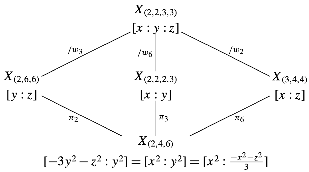
Ob­serve that, while the ca­non­ic­al mod­els for \( X_{(2,6,6)} \), \( X_{(3,4,4)} \) and \( X_{(2,2,2,3)} \) are pro­ject­ive lines over \( \mathbb{Q} \), each curve con­tains an el­lipt­ic point which is ra­tion­al only over a quad­rat­ic ex­ten­sion of \( \mathbb{Q} \). This ex­plains why \( (2,6,6) \) and \( (3,4,4) \) are not one of the sev­en \( \Gamma \)’s con­sidered be­fore. Non­ethe­less, us­ing the ex­pli­cit pro­jec­tions \( \pi_2, \pi_6, \pi_3 \) defined above, we can pull back the hy­per­geo­met­ric sheaf on \( X_{(2,4,6)} \) to sheaves on the three 2-fold cov­ers \( X_{(2,6,6)} \), \( X_{(3,4,4)} \) and \( X_{(2,2,2,3)} \) to ob­tain ex­pli­cit for­mu­lae of the traces of Hecke op­er­at­ors on the spaces of mod­u­lar forms for \( (2,6,6) \), \( (3,4,4) \) and \( (2,2,2,3) \) re­spect­ively, and then those for \( (2,2,3,3) \) by in­clu­sion and ex­clu­sion. See Sec­tion 7.1 of [e39] for more de­tail. Here we state the Hecke trace for­mula for \( \Gamma = (2,6,6) \) as an ex­ample.

We elab­or­ate more on the con­tri­bu­tions from el­lipt­ic points \( \lambda \in X_\Gamma(\mathbb F_p) \). When \( \lambda \) comes from the \( \mathbb{Q} \)-ra­tion­al el­lipt­ic point \( t=0 \) of \( (2,6,6) \) of or­der 2, \( \pi_2(0) \) is the el­lipt­ic point on \( X_{(2,4,6)} \) of or­der 4 and the con­tri­bu­tion de­pends on the be­ha­vi­or of \( p \) in \( \mathbb{Q}(\sqrt{-1}) \) as de­scribed by \eqref{eq_fo}. This is the unique el­lipt­ic point on \( X_\Gamma(\mathbb F_p) \) when \( -3 \) is a non­square \( \!\!\pmod p \). In this case there are \( p \) terms in the first sum, com­ing from \( \lambda \in P^1(\mathbb F_p), \lambda \ne 0 \). When \( -3 \) is a square \( \!\!\pmod p \), \( X_\Gamma(\mathbb F_p) \) has two more el­lipt­ic points, from \( t=\pm 1/\sqrt{-3} \), which are pro­jec­ted to the el­lipt­ic point of or­der 6 on \( X_{(2,4,6)} \) by \( \pi_2 \). Hence they give rise to the same con­tri­bu­tion, as de­scribed by the second rule in \eqref{eq_fo} since \( p \) splits in the CM field \( \mathbb{Q}(\sqrt{-3}) \). In this case the first sum con­sists of \( p-2 \) terms, com­ing from \( \lambda \in P^1(\mathbb F_p), \lambda \ne 0, \pm 1/\sqrt{-3} \).

Sim­il­ar res­ults can be ob­tained for oth­er suit­able sub­groups of \( (2,4,6) \) or with \( (2,4,6) \) re­placed by the oth­er six \( \Gamma \) stud­ied in The­or­ems 2 and 3.

Ex­pli­cit Hecke trace for­mu­lae have many ap­plic­a­tions. For in­stance, know­ing Hecke trace can lead to spe­cial val­ues of hy­per­geo­met­ric func­tions. As an ex­ample, it fol­lows from the reas­on­ing in Yang [e34] that the Hecke trace \( a_7(h_4^2) \) above yields the iden­tity \[ {}_3F_2\Biggl[\begin{matrix} \frac12 &\frac13 &\frac34\\ &\frac56 &\frac76 \end{matrix} ;\ \frac{2^{10}\cdot3^{3}\cdot5^{6}\cdot7}{11^{4}\cdot 23^4}\Biggr] =\frac{11\cdot 23}{140\sqrt 3} \,\frac{2^{1/3}(4+2\sqrt 2)}{7^{7/6}} \,\frac{\Gamma(7/6)\Gamma(13/24)\Gamma(19/24)}{\Gamma(5/6)\Gamma(17/24)\Gamma(23/24)}. \] The trace for­mu­lae in this pa­per are used by Grove in [e40] to ob­tain the ver­tic­al Sato–Tate dis­tri­bu­tion, as \( p \to \infty \), of the nor­mal­ized \( H_p(\operatorname{HD}(\Gamma); \lambda) \),  \( \lambda \in \mathbb F_p^\times \), for \( \Gamma \) of type (a). The dis­tri­bu­tion of that for \( \Gamma \) of type (b) can be ob­tained by a sim­il­ar idea.

Write \( X_\Gamma^\circ = X_\Gamma \setminus \{ \)cusps, el­lipt­ic points\( \} \). The auto­morph­ic sheaves \( V^k(\Gamma)_{\mathbb C} \) and \( V^k(\Gamma)_\ell \) on \( X_\Gamma \) are first defined on \( X_\Gamma^\circ \), then ex­ten­ded to \( X_\Gamma \) along the in­clu­sion \( \iota: X_\Gamma^\circ \to X_\Gamma \). The sheaves are first defined for \( \Gamma \) tor­sion-free, then use the push-for­ward to get sheaves for groups with tor­sion ele­ments. When \( \Gamma \) is tor­sion-free, the nat­ur­al map \( \mathfrak H \to X_\Gamma^{\circ} \) is a uni­ver­sal cov­er with cov­er­ing group \( \Gamma \) be­ing the fun­da­ment­al group \( \pi_1(X_\Gamma^{\circ}, *) \). If \( \Gamma \) is not tor­sion-free, then \( \Gamma \) mod its cen­ter is a quo­tient of \( \pi_1(X_\Gamma^{\circ}, *) \).

The group \( \operatorname{SL}_2(\mathbb R) \) acts on \( {\mathbb C}^2 \) ca­non­ic­ally and it gives rise to the ac­tion on \( \operatorname{Sym}^k ({\mathbb C}^2) \). Re­strict­ing to the sub­group \( \Gamma \) gives the ac­tion of \( \Gamma \) on \( \operatorname{Sym}^k ({\mathbb C}^2) \). For each in­teger \( k\ge 1 \), the com­plex sheaf \( V^k(\Gamma)_{\mathbb C} \) is a rank \( k+1 \) loc­al sys­tem on \( X_\Gamma \) defined by \[ V^k(\Gamma)_{\mathbb C} = \Gamma \backslash \bigl(\mathfrak H^* \times \operatorname{Sym}^k ({\mathbb C}^2)\bigr). \] The stalk at \( x \in X_\Gamma^\circ \) is \( \operatorname{Sym}^k ({\mathbb C}^2) \), that at \( x \) a cusp or el­lipt­ic point is \[ \bigl(\operatorname{Sym}^k ({\mathbb C}^2)\bigr)^{\Gamma_x}, \] the sub­space fixed by the sta­bil­izer \( \Gamma_x \) of \( x \) in \( \Gamma \). It was shown by Eichler [e3] and Shimura [e6] for \( \Gamma \) non-cocom­pact and by Kuga and Shimura [e7] for \( \Gamma \) cocom­pact that \[ H^1(X_\Gamma, V^k(\Gamma)_{\mathbb C}) \simeq S_{k+2}(\Gamma) \oplus \overline{S_{k+2}(\Gamma)}. \]

De­ligne [e13] and Ohta [e20] con­struc­ted, for each in­teger \( k \ge 1 \) and a prime \( \ell \), an \( \ell \)-ad­ic sheaf \( V^k(\Gamma)_\ell \) on \( X_\Gamma \otimes \overline {\mathbb Q} \) us­ing the mod­uli in­ter­pret­a­tion of \( X_\Gamma \). To ease our nota­tion, we use \( V^k(\Gamma)_{\ell, \bar \lambda} \) to de­note the stalk at the point \( \lambda \) of the sheaf \( V^k(\Gamma)_\ell \). For \( \Gamma \) el­lipt­ic mod­u­lar and tor­sion-free, \( V^k(\Gamma)_\ell \) has rank \( k+1 \). More pre­cisely, from the uni­ver­sal el­lipt­ic curve \( \mathcal E \) over \( X_\Gamma^\circ \), the stalk at an al­geb­ra­ic point \( \lambda \in X_\Gamma^\circ(K) \) over a num­ber field \( K \) is \[ V^k(\Gamma)_{\ell,\bar \lambda} = \operatorname{Sym}^{k}~ \bigl(V^1(\Gamma)_{\ell,\bar \lambda}\bigr), \] where \[ V^1(\Gamma)_{\ell, \bar \lambda} = H_{\text{ét}}^1(\mathcal E_\lambda \otimes \overline{\mathbb{Q}}, {\mathbb Q}_\ell) \] en­dowed with the ac­tion of \( \operatorname{Gal}(\overline {\mathbb{Q}}/K) \). In par­tic­u­lar, if \( \Gamma \) is el­lipt­ic mod­u­lar and \( -\operatorname{Id} \notin \Gamma \), then at \( \lambda \in X_\Gamma^\circ(\mathbb{Q}) \) we have, for all \( k \ge 1 \) and al­most all primes \( p \), \[ \operatorname{Tr} (\operatorname{Frob}_{p} | V^k(\Gamma)_{\ell,\bar {\lambda}}) = \sum_{j=0}^{\lfloor \frac k2 \rfloor }(-1)^j\binom{k-j}{j} p^j \operatorname{Tr} \bigl(\operatorname{Frob}_{p} | V^1(\Gamma)_{\ell,\bar {\lambda}}\bigr)^{k-2j}. \] This is the re­la­tion used in The­or­em 2.

For \( \Gamma \) arising from the in­def­in­ite non­split qua­ternion al­gebra \( B \) over \( \mathbb{Q} \) and tor­sion-free, \( V^k(\Gamma)_\ell \) has rank \( k+1 \) for \( k \) even. From the uni­ver­sal abeli­an sur­face over \( X_\Gamma \) with qua­ternion mul­ti­plic­a­tion by \( B \), at \( \lambda \in X_\Gamma(K) \) there is an \( \ell \)-ad­ic de­gree-2 rep­res­ent­a­tion \( \rho_{\ell,\lambda} \) of \( \operatorname{Gal}(\overline{\mathbb{Q}}/K) \) such that \[ V^{k}(\Gamma)_{\ell,\bar\lambda} = \operatorname{Sym}^{k}~ (\rho_{\ell,\lambda}), \] sim­il­ar to the el­lipt­ic mod­u­lar case. The rank of \( V^k(\Gamma)_\ell \) for \( k \) odd is very dif­fer­ent. For ex­ample, \( V^1(\Gamma)_\ell \) has rank 4. See ([e39], Sec­tion 2.2) for more de­tail.

If \( \Gamma \) con­tains \( -\operatorname{Id} \), be it el­lipt­ic mod­u­lar or qua­ternion­ic, \( V^{k}(\Gamma)_\ell \) and \( V^k(\Gamma)_{\mathbb C} \) are both zero for \( k \) odd; for \( k \ge 2 \) even, \( \lambda \in X_\Gamma^\circ(\mathbb{Q}) \), and al­most all primes \( p \), \[ \operatorname{Tr}\bigl(\operatorname{\operatorname{Frob}}_{p} | V^k(\Gamma)_{\ell,\bar {\lambda}}\bigr) = F_{k/2}\Bigl(\operatorname{Tr}\bigl(\operatorname{\operatorname{Frob}}_{p} | V^2(\Gamma)_{\ell,\bar {\lambda}}\bigr), p\Bigr), \] where \( F_m \) is defined by (2). This is the re­la­tion used in The­or­em 3.

Hence we only need to re­place \( V^2(\Gamma)_\ell \) or \( V^1(\Gamma)_\ell \) by a sheaf whose Frobeni­us traces are com­put­able. Our goal is to show that, for each of the sev­en tri­angle sub­groups \( \Gamma \) in Sec­tion 2.1, this can be achieved us­ing the hy­per­geo­met­ric sheaf as­so­ci­ated to \( \operatorname{HD}(\Gamma) = \{\alpha(\Gamma), \beta(\Gamma)\} \).

In this sub­sec­tion we in­tro­duce the hy­per­geo­met­ric sheaf, both com­plex and \( \ell \)-ad­ic, at­tached to a prim­it­ive hy­per­geo­met­ric datum \[ \operatorname{HD} = \{\alpha \,{=}\, \{a_1, \dots,a_n\}, \beta\,{=}\,\{b_1{=}1, b_2,\dots,b_n\}\} \] of length \( n \).

As we have seen in Sec­tion 2.2, the clas­sic­al hy­per­geo­met­ric func­tion as­so­ci­ated to \( \operatorname{HD} \) is \[_nF_{n-1}(\operatorname{HD}; z)= \sum_{r\ge 0} \prod_{1 \le i \le n}\frac{\Gamma(a_i+r)/\Gamma(a_i)}{\Gamma(b_i+r)/\Gamma(b_i)} ~z^r. \] Beuk­ers and Heck­man showed in [e23] that \( _nF_{n-1}(\operatorname{HD}; z) \) sat­is­fies the \( n \)-th or­der lin­ear or­din­ary dif­fer­en­tial equa­tion \begin{align*} & \bigl[\theta (\theta + b_2-1) \cdots (\theta + b_n-1) - z(\theta+a_1)\cdots (\theta+a_n)\bigr]F = 0,\\ & \theta = z \frac{d}{dz} \end{align*} which has three reg­u­lar sin­gu­lar­it­ies at \( 0, 1, \infty \) with loc­al ex­po­nents \[ \eqalign{ &0=1-b_1, 1-b_2,\dots, 1-b_n & \quad\text{ at } z&=0,\cr &a_1,\dots, a_n & \quad\text{ at } z&=\infty,\cr &0, 1,2,\dots, n-2, -1 + \textstyle\sum_{j} (b_j - a_j) & \quad\text{ at } z&=1. } \]

By as­sem­bling solu­tions of this dif­fer­en­tial equa­tion through the nonsin­gu­lar points we define a rank-\( n \) com­plex loc­al sys­tem on \( \mathbb P^1({\mathbb C})\setminus\{0, 1 \), \( \infty\} \). Fix a base point \( z_0 \in \mathbb P^1({\mathbb C})\setminus\{0, 1 \), \( \infty\} \). For \( i \in \{0, 1 \), \( \infty\} \), de­note by \( C_i \) a simple coun­ter­clock­wise loop start­ing and end­ing at \( z_0 \) en­clos­ing \( i \) and not the oth­er two sin­gu­lar­it­ies. Then \( \pi_1(\mathbb P^1({\mathbb C})\setminus\{0, 1 \), \( \infty\}, \) \( z_0) \) is gen­er­ated by the ho­mo­topy classes \( [C_0] \), \( [C_1] \), \( [C_\infty] \) with one re­la­tion \( [C_\infty][C_1][C_0] = \operatorname{Id} \). Let \( g_0, g_1 \), \( g_\infty \in \operatorname{GL}_n({\mathbb C}) \) be the mono­dromy ac­tion on the fiber at \( z_0 \) by ex­tend­ing solu­tions ana­lyt­ic­ally along \( C_0, C_1, C_\infty \), re­spect­ively.

The mono­dromy group of \( \operatorname{HD} \) is the tri­angle group \[ \langle g_0, g_1, g_\infty ~|~ g_\infty g_1 g_0 = \operatorname{Id} \rangle = ( e_0, e_1, e_\infty ), \] where \( e_i \) is the or­der of \( g_i \). The ei­gen­val­ues of \( g_\infty \) are \( e^{2\pi i a_j} \), those of \( g_0 \) are \( e^{-2\pi i b_j} \), while \( g_1 \) is a pseu­dore­flec­tion, that is, \( g_1-I_n \) has rank 1. This de­scribes the com­plex hy­per­geo­met­ric sheaf \( \mathcal H(\operatorname{HD})_{\mathbb C} \) on \( \mathbb P^1({\mathbb C})\setminus\{0, 1 \), \( \infty\} \) with the mono­dromy group \( ( e_0, e_1 \), \( e_\infty) \).

On the al­geb­ra­ic side, for each prime \( \ell \), Katz [e24], [e30] in­tro­duced an \( \ell \)-ad­ic rank-\( n \) hy­per­geo­met­ric sheaf \( \mathcal H(\operatorname{HD})_\ell \) on the mul­ti­plic­at­ive group \( \mathbb G_m \) with the ac­tion of \( \operatorname{Gal}(\overline {\mathbb{Q}}/\mathbb{Q}(\zeta_M)) \), where \( M =\operatorname{lcd}(\operatorname{HD}) \). Its ac­tion on the fiber at \( \lambda \in \mathbb{Q}(\zeta_M)^\times \) has Frobeni­us traces giv­en by hy­per­geo­met­ric char­ac­ter sums which are fi­nite field ana­log of \( {}_nF_{n-1}(\operatorname{HD};1/\lambda) \). When the datum \( \operatorname{HD} \) is defined over \( \mathbb{Q} \), that is, the set of the column vec­tors \[\Bigl\{ \Bigl(\,\begin{matrix} a_i\\b_i \end{matrix}\,\Bigr) \mod {\mathbb Z} \Bigr\} \] is in­vari­ant un­der mul­ti­plic­a­tion by ele­ments in \( (\mathbb Z/M\mathbb Z)^\times \), the Galois ac­tion at the fiber above \( \lambda \in \mathbb{Q}^\times \) can be ex­ten­ded to \( \operatorname{Gal}(\overline {\mathbb{Q}}/\mathbb{Q}) \). One such ex­ten­sion, de­noted \( \rho^{\operatorname{BCM}}_{\operatorname{HD},\lambda, \ell} \), was stud­ied by Beuk­ers, Co­hen and Mil­let [e36]. We sum­mar­ize key prop­er­ties of this rep­res­ent­a­tion be­low.

Here \( n-m \) is even, \( \delta = 1 \) when \( \sum a_i \equiv 1/2 \mod {\mathbb Z} \) and \( 2\| M \), and \( \delta=0 \) oth­er­wise. Moreover, the fam­ily of rep­res­ent­a­tions \[ \bigl\{\rho_{\operatorname{HD},\lambda,\ell}^{\operatorname{BCM}} : \text{prime }\ell\bigr\} \] of \( \operatorname{Gal}(\overline{\mathbb{Q}}/\mathbb{Q}) \) is com­pat­ible so that the trace of \( \operatorname{Frob}_p \) is in­de­pend­ent of the choice of \( \ell \ne p \).

There­fore, in or­der that \( V^2(\Gamma) \) or \( V^1(\Gamma) \) is iso­morph­ic to a hy­per­geo­met­ric sheaf or its twist by a char­ac­ter, the mod­u­lar curve \( X_\Gamma \) has to pos­sess the fol­low­ing prop­er­ties:

• \( X_\Gamma \) is defined over \( \mathbb{Q} \) and iso­morph­ic to \( \mathbb P^1 \);
• \( X_\Gamma \setminus X_\Gamma^\circ \) con­sists of three \( \mathbb{Q} \)-ra­tion­al points, which we may as­sume to be \( 0, 1, \infty \);
• \( \Gamma \) or \( \bar \Gamma :=\Gamma/\Gamma\cap \{\pm \operatorname{Id}\} \) is an arith­met­ic tri­angle group.

For the sev­en sub­groups \( \Gamma \) in Sec­tion 2.1, the mod­u­lar curves \( X_\Gamma \) meet these con­di­tions, and the data \( \operatorname{HD}(\Gamma)=\{\alpha(\Gamma) \), \( \beta(\Gamma)\} \) in Table 1 are defined over \( \mathbb{Q} \) so that The­or­em 5 ap­plies.

Let \( \Gamma=(e_0, e_1, e_\infty) \) be one of the sev­en tri­angle sub­groups in Sec­tion 2.1, and let \( \lambda = \lambda(\Gamma) \) be the para­met­er of the curve \( X_\Gamma \) tak­ing val­ues \( 0, 1, \infty \) at the three points of or­der \( e_0, e_1, e_\infty \), re­spect­ively. At a prime \( p \) where \( X_\Gamma \) has good re­duc­tion, \[ X_\Gamma(\mathbb F_p) = \mathbb P^1(\mathbb F_p) = \mathbb F_p \cup \{\infty\}. \] The con­tri­bu­tion to the trace of \( T_p \) on \( S_{k+2}(\Gamma) \) from a nonsin­gu­lar \( \lambda \in X_\Gamma(\mathbb F_p) \), namely \[ \lambda \in \mathbb F_p^\times, \quad \lambda \ne 1, \] fol­lows from the the­or­em be­low, in which \( \chi_d \) de­notes the quad­rat­ic char­ac­ter at­tached to \( \mathbb{Q}(\sqrt d) \), which we identi­fy as a char­ac­ter of \( \operatorname{Gal}(\overline {\mathbb{Q}}/\mathbb{Q}) \) by class field the­ory, or a char­ac­ter of \( \operatorname{Gal}(K/\mathbb{Q}(t)) \) trivi­al on \( \operatorname{Gal}(K/\overline{\mathbb{Q}}(t)) \) by (6).

To prove The­or­em 6, we take the geo­met­ric view­point ex­plained in Re­mark 2 to com­pare the auto­morph­ic sheaf and the hy­per­geo­met­ric sheaf oc­curred in (i) and (ii). Two gen­er­al res­ults are used. The first one is Katz’s ri­gid­ity the­or­em which com­pares two com­plex sheaves.

The table be­low shows that \( V^1(\Gamma)_{\mathbb C} \simeq \mathcal H(\operatorname{HD}(\Gamma))_{\mathbb C} \) for \( \Gamma \) of type (a): \begin{gather*} \begin{array}{|c|c|c|c|c|c|c|c|} \hline (e_0,e_1,e_\infty)&\text{Generators}& \text{Exponents}& {\operatorname{HD}(\Gamma)} & {\mathcal H(\operatorname{HD}(\Gamma))_{\mathbb C}}\\ \hline (\infty,\infty,3) & g_0=T:= \bigl({1 \atop 0}{1\atop 1}\bigr) & (1,1) & \alpha=\bigl\{\frac{1}{3}, \frac{2}{3}\bigr\} &\mathcal H\bigl(\bigl\{\frac1{3},\frac23\bigr\},\{1,1\}\bigr)_{\mathbb C}\\ \cong \Gamma_1(3) & g_1=S:= \bigl({-2 \atop -3}{3\atop4}\bigr) &(1,1)&\beta=\{1,1\}& \\ & g_\infty=(ST)^{-1} &\bigl(\frac13,\frac23\bigr)& &\\ \hline (\infty,\infty,\infty) & g_1=T:= \bigl({1\atop 0}{1\atop1}\bigr) & (1,1) &\alpha=\bigl\{\frac12, \frac12\bigr\} &\mathcal H\bigl(\bigl\{\frac1{2},\frac12\bigr\},\{1,1\}\bigr)_{\mathbb C}\\ \cong \Gamma_1(4) &g_0=(ST)^{-1} &(1,1)&\beta=\{1,1\} & \\ & g_\infty=S:= \bigl({1\atop4}{-1\atop-3}\bigr) &\bigl(\frac12,\frac12\bigr)& &\\ \hline \end{array} \end{gather*} A sim­il­ar table for type (b) groups shows \( V^2(\Gamma)_{\mathbb C} \simeq \mathcal H(\{\{1/2\},\{1\}\})_{\mathbb C} \otimes\mathcal H(\operatorname{HD}(\Gamma))_{\mathbb C} \).

Once the two com­plex sheaves are shown to be iso­morph­ic, the fol­low­ing com­par­is­on the­or­em says that their \( \ell \)-ad­ic coun­ter­parts may dif­fer at most by a twist by a char­ac­ter of \( \operatorname{Gal}(\overline{\mathbb{Q}}/\mathbb{Q}) \).

We then com­pare the two sheaves at a fiber to de­term­ine the twist char­ac­ter \( \chi_\Gamma \) for each \( \Gamma \).

It re­mains to com­pute the con­tri­bu­tions from the three sin­gu­lar points on \( X_\Gamma \). These are done sep­ar­ately and the cel­eb­rated Néron–Ogg–Sha­far­ev­ich cri­terion is used. At a cusp it is equal to 1 for \( k \) even, as done in Scholl [e22]; while for \( k \) odd, it is \( \pm 1 \) or 0 de­pend­ing on the type of re­duc­tion at \( p \) of the de­gen­er­ate el­lipt­ic curve rep­res­ent­ing the cusp. All el­lipt­ic points are CM points. We first de­term­ine the CM struc­ture at each el­lipt­ic point, then com­pute the con­tri­bu­tion at \( p \) from each el­lipt­ic point, which mainly de­pends on \( k \), the or­der of the point and the be­ha­vi­or of \( p \) in the CM field, as shown in The­or­ems 2 and 3.

Wen-Ching Win­nie Li re­ceived her Ph.D. from the Uni­versity of Cali­for­nia, Berke­ley in 1974, su­per­vised by An­drew P. Ogg. In 1979 she joined the Pennsylvania State Uni­versity, where she has been Dis­tin­guished Pro­fess­or of Math­em­at­ics since 2012.