by Kenneth Appel and Wolfgang Haken
In 1852, a few months after he had completed his studies at University College London, Francis Guthrie wrote a letter to his brother Frederick, who was still at the college as a student of the mathematician Augustus De Morgan. Francis pointed out to Frederick that it seemed that every map drawn on a sheet of paper can be colored with only four colors in such a way that countries sharing a common border have different colors. He asked if there was any way to prove this mathematically. Frederick did not know, and he asked De Morgan, who did not know either. For the next 124 years Guthrie’s four-color problem, the problem of proving that every map requires at most four colors or of drawing a map that requires five colors, intrigued professional mathematicians, amateur mathematicians and high school students who felt that all unsolved problems remain so only because of the incompetence of the older generation.
In 1976 we solved the four-color problem. Guthrie’s conjecture was proved mathematically, but in a way quite different from what he might have expected. Even among present-day mathematicians those who were not aware of the developments leading to the proof are rather dismayed by the result because the proof made unprecedented use of computers; the computations of the proof make it longer than has traditionally been considered acceptable. In fact, the correctness of the proof cannot be checked without the aid of a computer. Moreover, some of the crucial ideas of the proof were perfected by computer experiments. Of course, a short proof of the four-color theorem may some day be found, perhaps by one of those bright high school students. It is also conceivable that no such proof is possible. In this case a new and interesting type of theorem has appeared, one which has no proof of the traditional type.
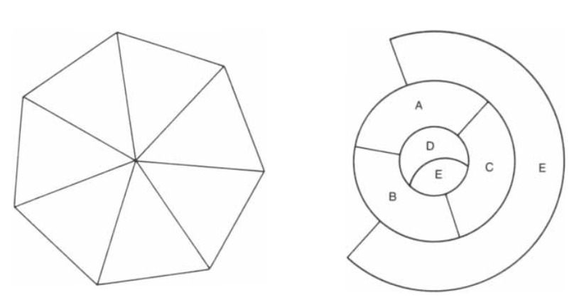
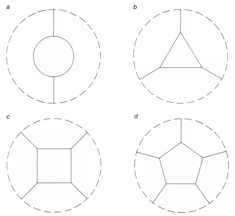
In spite of the novel aspects of the proof, both the four-color problem and the basic method of proof have deep roots in mathematics. We will begin to examine them by returning to the initial formulation of the problem in Francis Guthrie’s letter. By “neighboring” countries Guthrie must have meant countries adjacent along a borderline rather than at a single point; otherwise a map whose countries look like the wedges of a pie would require as many colors as there are countries. By “country” he certainly must have meant a connected region, because if a country is allowed to consist of more than one region and the regions are separate, it is not at all hard to construct an example of a map with five countries each of which is adjacent to each of the other four [see Figure 1].
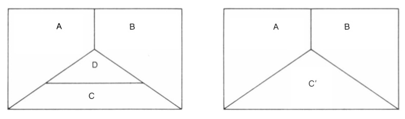
Guthrie and De Morgan certainly realized that a map with four countries can be drawn in which each country is adjacent to the other three [see Figure 2, left]. Such a map requires four colors and therefore a three-color conjecture is false. Three colors will not suffice to color all maps.
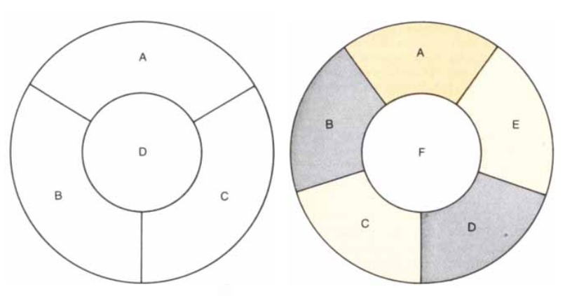
De Morgan proved that it is not possible for five countries to be in a position such that each of them is adjacent to the other four. This led him to believe that five colors would never be needed and thus that the four-color conjecture was true. Proving that five mutually adjacent countries cannot exist in a map does not prove the four-color conjecture, however [see Figure 2]. Many amateur mathematicians, not understanding this fact, have independently discovered proofs of De Morgan’s result and have then thought that they had proved the four-color conjecture.
In 1878 the mathematician Arthur Cayley, unable to prove or disprove the four-color conjecture, presented the problem to the London Mathematical Society. Less than a year later Alfred Bray Kempe, a barrister and member of the society, published a paper purporting to show that the conjecture is true. Kempe’s argument was extremely clever, and although his proof turned out to be incomplete, it contained most of the basic ideas that led to the correct proof a century later. Kempe tried to prove the conjecture true by the classical method of reductio ad absurdum; he assumed that the conjecture is false (that is, that there is at least one map which requires five colors) and then proceeded to show that this assumption leads to a contradiction. Reaching a contradiction shows that the original assumption (some maps require five colors) is wrong and therefore the four-color conjecture (four colors are always enough) is true.
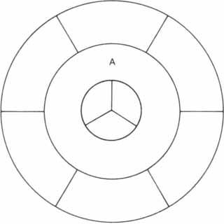
Kempe began by defining normal maps: A map is normal if none of its countries enclose other countries and if no more than three countries meet at any point [see Figure 3]. He then showed that if there were a map that required five colors, a “five-chromatic” map, then there would have to be a normal five-chromatic map. Thus to prove the four-color conjecture it is sufficient to prove that a normal five-chromatic map is not possible. Kempe noted that if there were a normal five-chromatic map, then there would have to be such a map with a smallest number of countries, a “minimal normal five-chromatic” map. (In other words, any map with fewer countries than the minimal five-chromatic map can be colored with four or fewer colors.) Therefore to prove the four-color conjecture it is sufficient to prove that a minimal normal five-chromatic map is impossible, that is, that postulating the existence of a minimal normal map requiring five colors leads to a contradiction.
Kempe approached a contradiction as follows. He proved that any normal map must have some country with five or fewer neighbors. He then argued that if a minimal normal five-chromatic map has a country with fewer than six neighbors (which, as he had just shown, every normal map must have), then there would have to be a normal map with fewer countries that is also five-chromatic. If this argument had been totally correct, a contradiction would have been reached. By assuming the existence of a minimal five-chromatic map Kempe would have proved the existence of a smaller five-chromatic map. That would contradict the definition of a minimal five-chromatic map, and so no such map would be possible. Since that implies that there can be no five-chromatic map at all, the proof would have been complete. Kempe proved correctly that a country with two, three or four neighbors existing in a minimal five-chromatic map leads to a contradiction, but his proof of the case of five neighbors was faulty. In our proof of the four-color theorem we corrected Kempe’s flawed analysis of the last case by examining some 1,500 arrangements of countries. Our methods were basically extensions of valid parts of Kempe’s proof that have been the object of great attention and refinement by mathematicians over the past 100 years.
Kempe had shown that in every normal map there is at least one country with two, three, four or five neighbors. (In other words, there are no normal maps on a plane in which every country has six or more neighbors.) This may be expressed by the statement that the set of “configurations” consisting of a country with two neighbors, a country with three neighbors, a country with four neighbors and a country with five neighbors [see Figure 5] is “unavoidable,” that is, every normal map must contain at least one of these four configurations. Unavoidability is one of the two important ideas that are basic to our proof of the four-color theorem.
The second important idea is reducibility. A configuration is intuitively reducible if there is a way of showing, solely by examining the configuration and the way in which chains of countries can be aligned, that the configuration cannot possibly appear in a minimal five-chromatic map. Kempe showed that three of his four configurations are reducible but failed to show that a country with five neighbors is a reducible configuration. The methods of proving configurations reducible grew out of Kempe’s proof that a country with four neighbors cannot occur in a minimal five-chromatic map. The use of the word reducible stems from the form of Kempe’s argument; he proved that if a minimal five-chromatic map contains a country with, say, four neighbors, then there is a five-chromatic map with a reduced number of countries [see Figure 6 and Figure 7].
We can describe Kempe’s attack on the four-color conjecture as an attempt to find an unavoidable set of reducible configurations. Finding such a set is sufficient for proving the four-color conjecture because it shows that every map contains a configuration that cannot be part of a minimal five-chromatic map. Therefore there can be no minimal five-chromatic map, and as Kempe proved correctly this implies that there can be no five-chromatic map at all. Like Kempe, we attacked the four-color problem by constructing an unavoidable set of reducible configurations. Instead of four simple configurations, however, our set consisted of some 1,500 complex figures.
In 1890, 11 years after Kempe published his proof, Percy John Heawood pointed out that Kempe’s argument that no minimal five-chromatic map could contain a country with five neighbors was flawed, and that the error did not appear easy to repair. In his attack on the problem Heawood investigated a generalization of the original four-color conjecture. The maps studied by Guthrie and Kempe were maps in a plane or on a sphere. Heawood, considering maps on more complicated surfaces, was able to obtain an elegant argument that provided an upper bound for the number of colors required to color maps on these surfaces. If the method he used had been applicable to the plane, it would have provided a proof of the four-color conjecture.
Heawood continued to work on the problem for no less than 60 years. During that time many other eminent mathematicians devoted a great deal of effort to the four-color conjecture. One may wonder why so many mathematicians would spend so much time on what appeared to be a question of so little practical significance. The explanation lies in the discoveries made about the nature of pure mathematics over the past century and in the effect of those discoveries on the faith of mathematicians in the power of mathematics.
Toward the end of the 19th century mathematicians were able to build powerful theories that enabled them to settle many difficult questions. The feeling grew that any question that could be reasonably posed in the language of mathematics could be answered by the use of sufficiently powerful mathematical ideas. Moreover, it was believed that these questions could be answered in such a way that a competent mathematician could check the correctness of the answer in a reasonable length of time. The four-color conjecture certainly appeared to be such a problem. If mathematicians could not solve the problem, it seemed clear that they had simply not yet developed the appropriate mathematical tools.
In the 1930’s, however, new discoveries challenged the 19th-century faith in the completeness of mathematics. Kurt Gödel and Alonzo Church obtained new and disturbing results in formal logic, the branch of mathematics in which the concept of proof is stated most precisely. It was proved that in what seems to be the most natural logical system there are true statements that cannot be proved true (or false) in the system. Moreover, there are theorems in the system with relatively short statements whose shortest proofs are too long to be written down in any reasonable length of time. In the 1950’s further investigation showed that the same difficulties affect branches of mathematics other than logic. Some mathematicians began to think that the four-color conjecture might be one of those statements that can neither be proved nor disproved; after all, the conjecture had been studied without success for 80 years. Other workers felt that if a proof existed, it would be too long to write down. Many believed, however, that the disease of unsolvability could not spread to this area of mathematics and that an elegant mathematical argument would be found to decide the truth or falsehood of the four-color conjecture.
We now know that a proof can be found. But we do not yet know (and may never know) whether there is any proof that is elegant, concise and completely comprehensible by a human mathematical mind. So many areas of mathematics have been involved in various attempts to prove the four-color conjecture that it would be impossible to discuss them all here. We shall restrict our attention to work that led directly to the proof.
In 1913 George D. Birkhoff of Harvard University improved on Kempe’s reduction technique and was able to show that certain configurations larger than Kempe’s were reducible. Philip Franklin of the Massachusetts Institute of Technology utilized some of Birkhoff’s results to show that a map requiring five colors must have at least 22 countries, that is, that any map with fewer than 22 countries is four-colorable. Birkhoff’s methods were improved by many mathematicians between 1913 and 1950. During this period reducible configurations were exploited primarily to improve Franklin’s result; by 1950 it had been shown that any map with fewer than 36 countries is four-colorable.
Although the work in this area did show that many configurations are reducible, the set of all the configurations that had been proved reducible by 1950 did not even come close to forming an unavoidable set. Only a few mathematicians had constructed unavoidable sets of configurations, and there was little hope that their work would lead to an unavoidable set of reducible configurations.
Heinrich Heesch of the University of Hannover seems to have been the first mathematician after Kempe to publicly state that the four-color conjecture could be proved by finding an unavoidable set of reducible configurations. Heesch, who began his work on the conjecture in 1936, made several major contributions to the existing theory. In 1950 he estimated that the reducible configurations in the (then) hypothetical unavoidable set would be of certain restricted sizes and number about 10,000.
Configuration size must be a major consideration in this approach to the four-color problem. In the century since Kempe first introduced the idea of reducibility certain standard methods for examining configurations to determine whether or not they are reducible have been developed. Employing these methods to show that large configurations are reducible requires the examination of a large number of details and appears feasible only by computer. Every configuration is surrounded by a ring of neighbors; the ring size, or number of countries that form the ring around the configuration, has a direct bearing on the difficulty of proving the configuration reducible. When one is trying to construct an unavoidable set of reducible configurations and discovers that a particular configuration is not reducible, one can often replace it to good effect with one or more other configurations, usually configurations of a larger ring size. Replacing one configuration with another whose ring contains an additional vertex, however, greatly increases the difficulty of reducibility testing and the computer time needed for it. This is in part because the number of distinct proper colorings of the vertices of the new ring is about three times the number of colorings of the vertices in the original ring. Furthermore, programs to test reducibility consider each possible coloring several times. In 1950 the difficulties of computation seemed to rule out the possibility of producing an unavoidable set of configurations and proving that each of its members is reducible.
With the advent of high-speed digital computers, however, an attack on these problems became technically possible. Heesch formalized the known methods of proving configurations reducible and observed that at least one of them (a straightforward generalization of the method used by Kempe) was in principle a sufficiently mechanical procedure to be implemented by computer. Heesch’s student Karl Dürre then wrote a computer program that used this procedure to prove configurations reducible. Whenever such a program succeeds in proving a configuration reducible, the configuration is certainly reducible. A negative result, however, shows only that the particular method of proving reducibility is not sufficient to prove the configuration reducible; it might be possible to prove it reducible by other methods. In some cases, when Dürre’s program failed to prove a configuration reducible, Heesch succeeded. He was able to show the configurations reducible with data generated by the program and with further calculations using a stronger technique developed by Birkhoff.
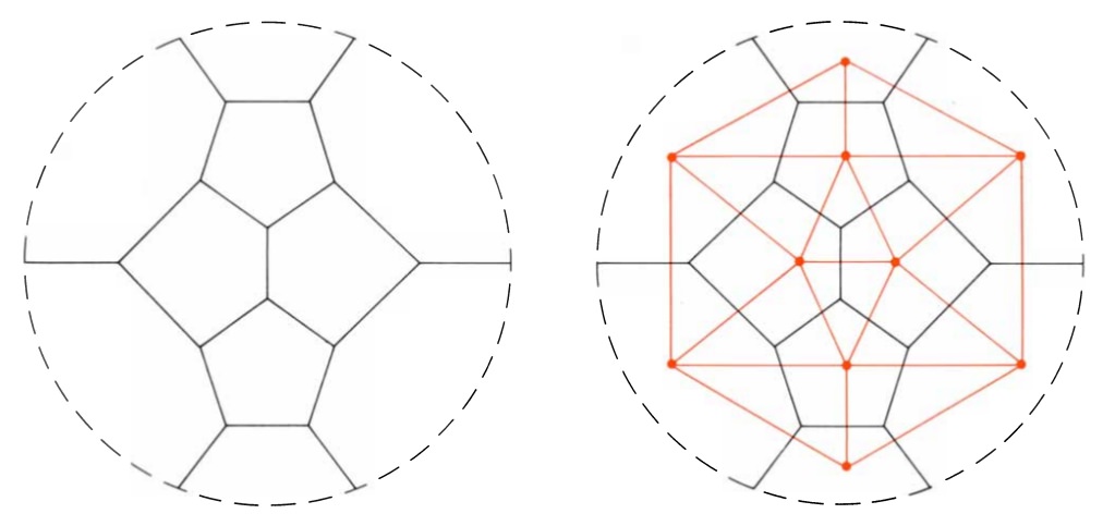
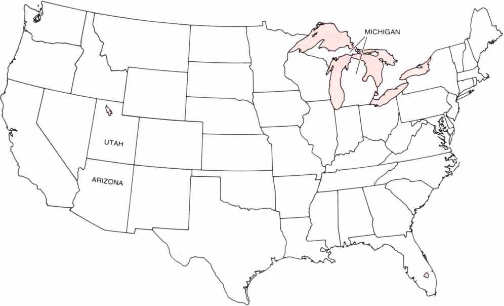
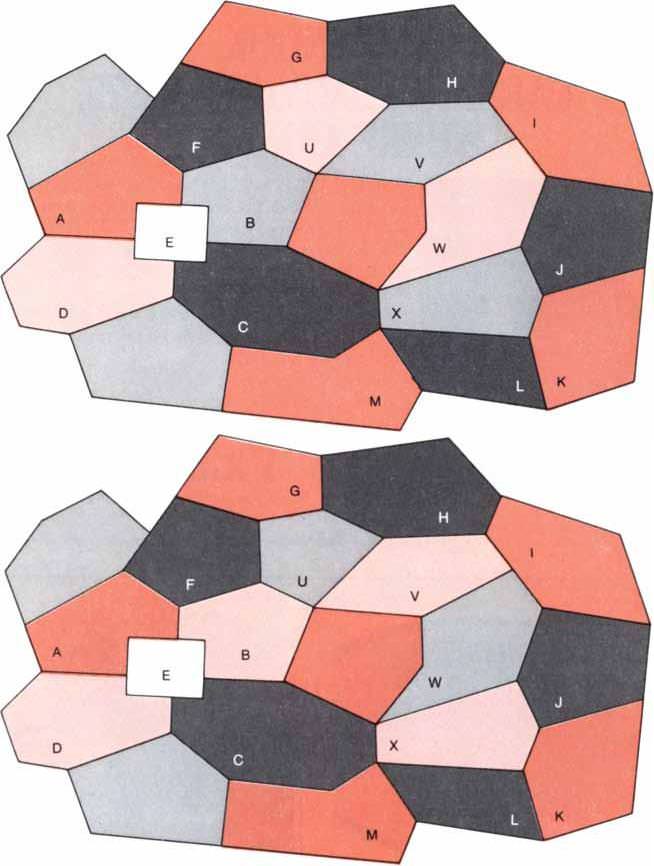
Heesch described configurations in a convenient way. He began by transforming the original map into what mathematicians call a dual form: a planar graph in which each vertex of the graph represents a country and each line segment between vertices represents a border. To obtain a dual graph of a map mark the capital in each country in the map and then, whenever two countries are neighbors, join their capitals by a road across the common border [see Figure 8]. Now remove everything except the capitals (called vertices) and the roads (called edges) you have added. These vertices and edges form the dual graph of the original map. The edges of a graph divide the plane into regions that are called faces. If the original map is normal (and only normal maps must be considered in the proof of the four-color theorem), all of the faces are triangles. In this case the dual graph is called a triangulation. The number of edges that end at a particular vertex (in the dual graph) is called the degree of the vertex and is equal to the number of neighbors of the country (in the original map) that is represented by that vertex. A path of edges that starts and ends at the same vertex and does not cross itself separates the graph into two parts: its interior and its exterior. Such a path is called a circuit.
In the vocabulary of dual graphs a configuration is a part of a triangulation consisting of a set of vertices plus all of the edges joining them. The boundary circuit, consisting of those vertices adjacent to the configuration and the edges joining them, is called the ring of the configuration. (The ring in the graph corresponds to the ring of countries that bound the configuration in the original map.) Configurations are often described by the lengths of their rings: a six-ring configuration, for example, is one whose boundary circuit has exactly six vertices.
With Heesch’s work the theory of reducible configurations seemed extremely well developed. Although certain improvements in the methods of proving reducibility have since been made, all of the ideas on reducibility that were needed for the proof of the four-color theorem were understood in the late 1960’s. Comparable progress had not been made in finding unavoidable sets of configurations. Heesch introduced a method that was analogous to moving charge in an electrical network to find an unavoidable set of configurations (not necessarily reducible), but he had not treated the idea of unavoidability with the same enthusiasm as the idea of reducibility. This method of “discharging” that first appeared in rather rudimentary form in the work of Heesch has been crucial, however, in all later work on unavoidable sets. In a much more sophisticated form it became the central element in the proof of the four-color theorem; hence we will explain it in some detail.
Kempe’s work shows that a triangulation that represents a minimal five-chromatic map cannot have any vertices with fewer than five neighbors. Thus in what follows we will for convenience use the word triangulation to mean a triangulation with no vertices of degree less than five. If we assign the charge number 6-\( k \) to every vertex of degree \( k \) (that is, with \( k \) neighbors), then vertices of degree greater than six (major vertices) are assigned negative charge and only vertices of degree five are given positive charge. It follows from Kempe’s work that the sum of the assigned numbers of any triangulation is exactly 12. This somewhat surprising result depends both on the fact that the graph is drawn in the plane and that it is a triangulation. The particular sum of 12 is not very important. What is extremely important is that for every planar triangulation this charge sum is positive.
Now suppose the charges in such a triangulation are redistributed, moved around without losing or gaining charge in the entire system. In particular suppose positive charge is moved from some of the positively charged (degree-five) vertices to some of the negatively charged (major) vertices. It is certainly not possible to change the (positive) sum of the charges by these operations, but the vertices having positive charge may change; for example, some degree-five vertices may lose all positive charge (become discharged), whereas some major vertices may gain so much charge that they end up with positive charge (become overcharged). Different vertices become discharged or overcharged according to the discharging, or redistribution, procedure chosen.
Given a specified discharging procedure on an arbitrary graph, however, it is possible to make a finite list of all the configurations that, after discharging is done, have vertices of positive charge.
(Of course, each of these configurations can be repeated an unforeseeable number of times.) In other words, positive charge can only occur within this finite set of configurations. Since the total charge is always positive, there will always be some vertices of positive charge. Therefore since all possible receptacles of positive charge are included in the list of configurations, every planar triangulation must contain at least one of these configurations. This process — generating a list of specific configurations from an arbitrary map — works because it is possible to determine the layout of small pieces of the map without knowing the form of the complete map.
In the proof of the four-color theorem the purpose of this discharging of positive vertices is to find a procedure describing exactly how to move charge in such a way as to ensure that every vertex of positive charge in the resulting configuration must either belong to a reducible configuration or be adjacent to one. Since the configurations signaled by this procedure must form an unavoidable set, if they are also reducible, then the four-color conjecture is proved. Of course, if not all of the resulting configurations are reducible, then no real progress has been made. In fact. Kempe’s unavoidable set can be considered to be the one resulting from the ineffective procedure of moving no charges at all.
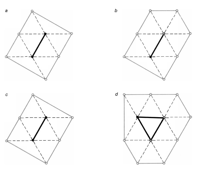
An example of a rather simple discharging procedure and the associated unavoidable set may make these ideas clearer. Consider the procedure that transfers 1/5 unit of charge from every degree-five vertex to each of its major neighbors [see Figure 9]. The corresponding unavoidable set consists of two configurations. One is a pair of degree-five vertices joined by an edge and the other is a degree-five vertex joined by an edge to a degree-six vertex.
These configurations are obtained as follows. A degree-five vertex can only end up positive in this procedure if at least one of its neighbors is not major, so that the vertex is forced to retain positive charge; the vertex either has a degree-five neighbor (the situation corresponding to the first configuration in the set) or a degree-six neighbor (the second configuration).
A degree-six vertex starts with no charge and therefore cannot receive any. A degree-seven vertex can only become positive if it has at least six neighbors that are degree-five vertices; if it has at least six such neighbors, two of them are joined by an edge (the first configuration of the unavoidable set). A vertex of degree eight or higher cannot become positive even if all of its neighbors are degree-five vertices. This can be seen by examining a degree-eight vertex. Its charge is minus two and the maximum positive charge it can receive is eight times 1/5, or 1 3/5. Thus the two (nonreducible) configurations form an unavoidable set; that is, since these calculations apply to any planar triangulation (with no vertices of degree less than five) a member of the two-configuration set will be found in every such triangulation of the plane.
In 1970 one of us (Haken) noticed certain methods of improving discharging procedures and began to hope that such improvements might lead to a proof of the four-color conjecture. The difficulties, however, still appeared to be formidable. One was that it was believed that very large configurations (with rings of neighbors containing as many as 18 vertices) would be included in any unavoidable set of reducible configurations. This meant that the problem might be beyond the capabilities of existing computers because although testing configurations of small ring size (up to about 11 vertices) for reducibility was reasonably simple on a computer, the computer time required increased by a factor of four for every unit increase in ring size. To make things worse, the computer storage requirements increased just as quickly. When Dürre’s program was applied to a particularly difficult 14-ring configuration, it took 26 hours to prove that the configuration did not satisfy even the most mechanical definition of reducibility (the definition stated with the fewest machine instructions). Even if the average time required to examine a 14-ring configuration were only 25 minutes, testing an average 18-ring configuration would require \( 4^4 \times 25 \) minutes, or more than 100 hours, of computer time and more storage than was available on any existing computer.
Another major difficulty was that no one really knew how many reducible configurations would be needed to form an unavoidable set. It seemed likely that the number of configurations would be in the thousands, but no upper limit had been established. Suppose that on a computer with sufficient storage it takes 100 hours to show that an 18-ring configuration is reducible. If there are 1,000 18-ring configurations in the set, it would take 100,000 hours, or more than 11 years, to prove them reducible on a very large computer. For all practical purposes if the set had been that large, the proof would have had to wait for computers much faster than those currently available.
Even if the theorem could be proved by finding an unavoidable set of reducible configurations, the proof would not satisfy those who demand mathematical elegance. What would be even more upsetting to many mathematicians, no one would be able to check the reducibility of all the configurations in the set by hand. By 1970, however, many experts on the four-color problem were quite pessimistic about finding a short proof. The problem had received a great deal of attention since its formulation more than 100 years earlier. Many approaches to the problem had been tried, but although some had led to important results in other areas of mathematics, none had ever led to a proof of the four-color theorem.
When we began our work on the problem in 1972, we felt certain that the techniques available to us would not lead to a noncomputer proof. We were even quite doubtful that they could lead to any proof at all before much more powerful computers were developed. Therefore our first step in attacking the problem of finding an unavoidable set of reducible configurations was to determine whether or not there was any hope of finding such a set with configurations of ring size sufficiently small that the computer time for the proofs of reducibility would be within reason. By the very nature of this question it was clear that we should not begin by examining the reducibility of all the configurations considered; otherwise the time spent in making the estimate would exceed the expected time needed for the entire task.
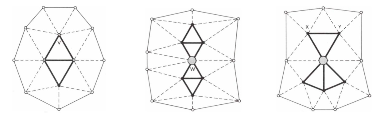
Here a thought of Heesch’s proved extremely useful. While he was testing configurations for reducibility he observed a number of distinctive phenomena that provide clues to the likelihood of successful reduction. For example, there are certain conditions involving the neighbors of vertices of a configuration under which no reducible configuration had ever been found. No reducible configuration had ever been found that contained, for instance, at least two vertices, a vertex adjacent to four vertices of the ring and no smaller reducible configurations. Although no proof is known that reducible configurations with these reduction obstacles could not exist, it seemed prudent to assume that if one wanted reducible configurations, one should avoid such configurations. Heesch found three major reduction obstacles, including the one described above, that could be easily described [see Figure 10]. No configuration containing one of them has ever been proved to be reducible.
It is easy to determine whether or not a configuration contains a reduction obstacle, and configurations without reduction obstacles have a very good chance of being reducible. If there was a manageable unavoidable set of configurations free of reduction obstacles, we felt there would have to be an unavoidable set of roughly the same size containing only reducible configurations.
We therefore decided to first study certain kinds of discharging procedure in order to determine the types of sets of obstacle-free configurations that might arise. To gain an understanding of what was needed, even for this study, we restricted the already restricted problem to what are called geographically good configurations: configurations that do not contain the first two of Heesch’s three obstacles.
In the fall of 1972 we wrote a computer program that would carry out the particular type of discharging procedure that seemed most reasonable to us. We were not ready to prove the theorem, so that the output of our program was not an unavoidable set but rather a list of the configurations that resulted from the most important situations. Although a computer program could not be expected to proceed as cleverly as a human being, the immense speed of the computer made it possible to accept certain inefficiencies. In any event the program was written in such a way that its output could be easily checked by hand.

The first runs of the computer program in late 1972 gave us a great deal of valuable information. First, it appeared that geographically good configurations of reasonable size (with a ring size of no more than 16) would be found close to most vertices of ultimately positive charge. Second, the same configurations occurred frequently enough for it to appear that the list of configurations might be of manageable length. Third, as the procedure was originally organized the computer output was too large to handle; similar cases repeated the same argument too often. Fourth, there were clearly some flaws in the procedure, since there were vertices of ultimately positive charge in whose neighborhoods no geographically good configurations could be guaranteed. Finally, the program generated a tremendous amount of information in only a few hours of computer time, so that we knew it would be possible to experiment often.
The program and certain aspects of the discharging procedure had to be modified to overcome the problems indicated by the first computer runs. Since we could preserve the basic program structure, the changes were not too difficult to make, and a month later we made a second set of runs. Now that the major problems had been corrected, we could perceive subtler problems. After some study we found solutions to these problems and again modified the program.
The man-machine dialogue continued for another six months until we felt that our procedure would obtain an unavoidable set of geographically good configurations in a reasonable amount of time. At this point we decided to prove formally that the procedure would provide a finite unavoidable set of geographically good configurations. We had to put aside the experimental approach and describe the total procedure. It was necessary to prove that all cases had been covered and that those cases that were not handled by the computer program were as simple as they appeared to be.
Much to our surprise this task proved extremely difficult and took more than a year. It was necessary to formulate general definitions of terms and to prove abstract statements about them. Special cases, even those that were not likely to arise in practice, had to be examined in detail and often required complicated analyses. Finally, by the fall of 1974, we had a lengthy proof that a finite unavoidable set of geographically good configurations does exist, and we had a procedure for constructing such a set with precise, although much larger than desirable, bounds on the size of the configurations in the set. The procedure we had designed was extremely important to us because we intended to apply it in the proof of the four-color theorem. (A short time later Walter Stromquist, a major contributor to reduction theory who was then a graduate student at Harvard, devised an elegant proof of the existence of unavoidable sets of geographically good configurations. Since Stromquist’s proof did not provide a method of actually constructing the configurations in the set, however, it appeared unlikely that it would be immediately applicable to the four-color conjecture itself.)
When we had proved that our procedure would work for geographically good configurations, we still did not know how complicated carrying out the procedure would be. We decided to try it on the restricted problem of triangulations having no pairs of adjacent degree-five vertices. This, of course, is a strong restriction, but the unavoidable set of geographically good configurations we obtained was quite small: only 47 configurations and none of them of a ring size larger than 16. We guessed that the solution to the unrestricted problem might be 50 times more unwieldy (this turned out to be a bit optimistic), and we decided that there was good reason to continue. Early in 1975 we modified the program so that it produced obstacle-free configurations rather than geographically good ones and forced it to search for sets in which more of the configurations had small ring size. When we ran the modified program, certain flaws became evident but there was also a very pleasant surprise: Replacing geographically good configurations with obstacle-free ones only doubled the size of the unavoidable set.
At this point the program, which had been absorbing our ideas and improvements for two years, began to surprise us. When we had hand-checked the analyses produced by the early versions of the program, we were always able to predict their course, but now the computer was acting like a chess-playing machine. It was working out compound strategies based on all the tricks it had been taught, and the new approaches were often much cleverer than those we would have tried. In a sense the program was demonstrating superiority not only in the mechanical parts of the task but in some intellectual areas as well.
By the summer of 1975 we believed that there was a good chance that we could find an unavoidable set of configurations each of which would be obstacle-free and likely to be reducible. Such a set would certainly contain some irreducible configurations, but we felt that by some small change of procedure we would be able to replace them with reducible configurations. Now for the first time we would have to test configurations for reducibility.
We began by writing a program to test for the most mechanical reducibility, working with the assembler language for the University of Illinois IBM 360 computer. We had been joined the preceding fall by John Koch, a graduate student in computer science who chose to write a dissertation on the reducibility of configurations of small ring size. (Frank Allaire of the University of Manitoba and Edward Swart of the University of Rhodesia were doing somewhat similar work of which we were unaware.) By the fall of 1975 Koch had written programs to check for the most mechanical reducibility in configurations of a ring size up to 11 and had gone on to more general investigations.
Over the next few months, with Koch’s aid, we modified his work on 11-ring configurations to produce programs for checking the reducibility of 12-, 13- and 14-ring configurations. Finally we further modified these programs to apply a more general procedure for reduction that had been developed by Birkhoff.
At this point our work on the discharging procedure reached an impasse. Structural changes, not just adjustments of parameters and small additions, were required to improve the program, and each change would mean a major modification of it. We therefore decided to discard the program and implement the discharging procedure by hand. This would ensure greater flexibility and allow the procedure to be modified locally whenever necessary. In December, 1975, we made an encouraging discovery. One of the rules that defined our discharging procedure was too rigid. Relaxing the rule made the procedure considerably more efficient.
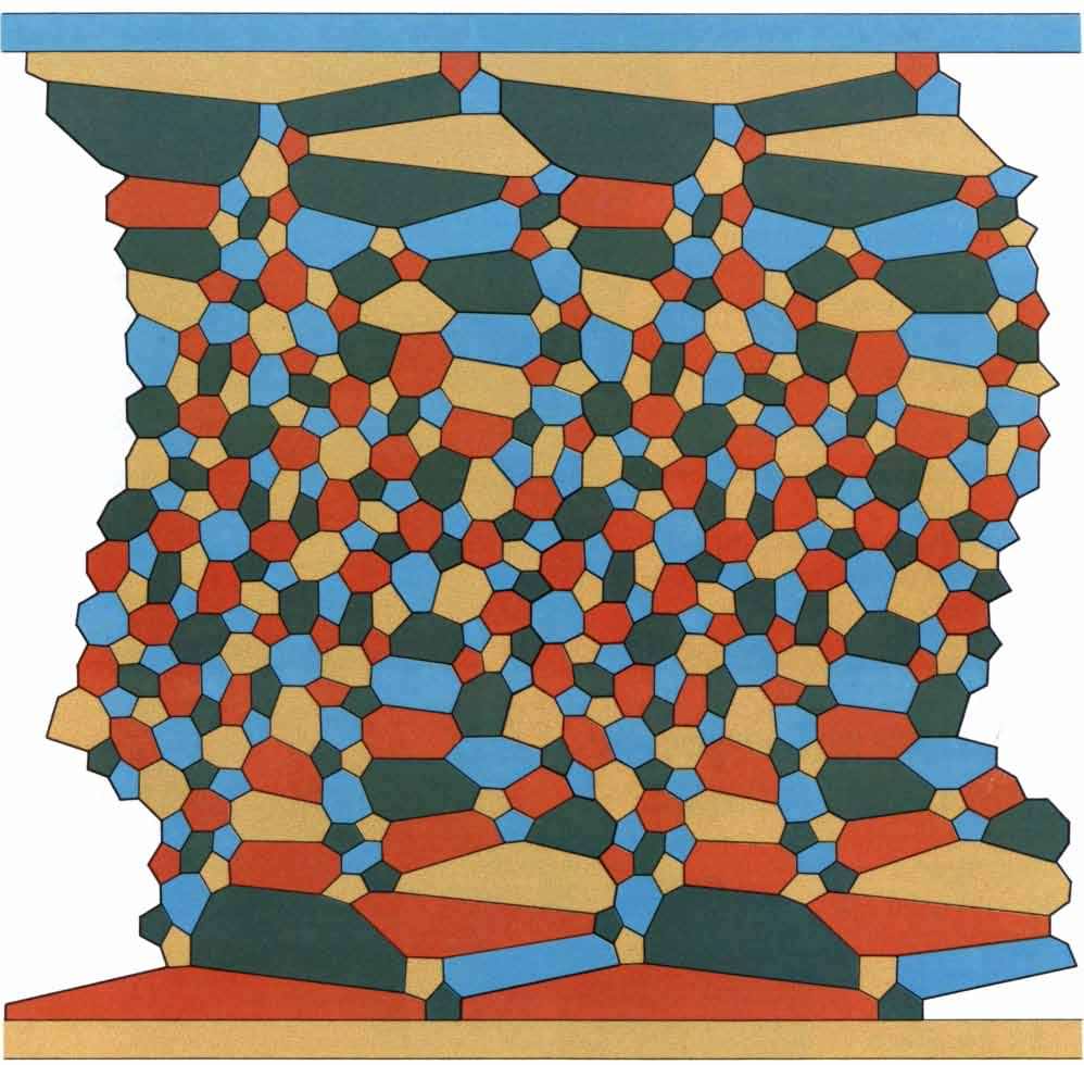
With the new discharging procedure it looked as though we could build an unavoidable set whose reducible configurations would be smaller than those produced by earlier procedures. The computer time required for the proof would probably be less than previous estimates indicated. It was still evident, however, that a considerable computational effort would be required to produce even the best unavoidable set of reducible configurations. Edward F. Moore of the University of Wisconsin had developed a powerful method for constructing maps that contained no small reducible configurations. For example, he had created a map in which the ring size of the smallest reducible configuration is 12 [see Figure 12]. Therefore any unavoidable set of reducible configurations must have at least one configuration of ring size 12. Moore’s work provides a lower bound on ring size, but we now feel sure that a ring size of 13 is necessary, and it is quite likely that a ring size of 14 is also necessary. (Our proof demonstrates that no larger configurations are needed.)
In January, 1976, we began the construction of an unavoidable set of reducible configurations by means of our new discharging procedure. The final version of the procedure had one further advantage for ensuring the reducibility of the final configurations. The procedure was essentially self-modifying; the program was designed to identify critical, or problem, areas — configurations that looked as though they would resist reduction efforts — and to modify itself to move positive charge to a different place. Since we were doing the discharging procedure without the computer, we knew that the procedure could be modified as we encountered critical areas.
We began by making an approximation, a preliminary run of our discharging procedure. We considered each possible case in which a vertex was forced to be positive, and in each case the neighborhood was examined to find an obstacle-free configuration. If none was found, the neighborhood was called critical, which meant that the discharging would have to be modified to avoid this problem. Even when an obstacle-free configuration was found, however, we could not guarantee a reducible configuration. The new reduction programs were used to try to find some obstacle-free configuration in the neighborhood that was also reducible. If none was found, the neighborhood was also called critical.
This method of developing an unavoidable set of reducible configurations (as we perfected a discharging procedure) was only possible by another dialogue with the computer. To determine which neighborhoods were critical it was necessary to check for reducibility quickly, in terms of computer time and in terms of real time. Fortunately it was seldom necessary to wait more than a few days for results, even though often a considerable amount of computer time was needed. Since this intensive man-machine interaction was indispensable to our work, we should explain the circumstances that made it possible.
Although our arrangement for computer usage seemed quite natural to us at the time, we have since discovered that we were indeed fortunate to be working at the University of Illinois, where a combination of a large computing establishment and an enlightened policy toward the research use of computers gave us an opportunity that seems to be unavailable at almost any other university or research establishment. Although we could not guarantee that our work would lead to a proof of the four-color theorem, we were given well over 1,000 hours of computer time in what we feel was an admirable display of faith in the value of pure mathematical research. We were informed by the computer center that because the university’s computers were not fully utilized at all times by class work and other kinds of research we could be included in a small group of computer users who were allowed to share the surplus computer time. We now know that this policy was essential to our success.
In June, 1976, we completed our construction of an unavoidable set of reducible configurations. The four-color theorem was proved. We had used 1,200 hours of time on three different computers. The final discharging procedure differed from our first approximation by some 500 modifications resulting from the discovery of critical neighborhoods. The development of the procedure required the hand analysis of some 10,000 neighborhoods of vertices of positive charge and the machine analysis of more than 2,000 configurations. A considerable part of this material, including the reduction of 1,482 configurations, was used in the final proof. Although the discharging procedure (without the reductions) can be checked by hand in a couple of months, it would be virtually impossible to verify the reduction computations in this way. In fact, when we submitted our paper on the proof to Illinois Journal of Mathematics, its referees checked the discharging procedure from our complete notes but checked the reducibility computations by running an independent computer program.
Many mathematicians, particularly those educated before the development of high-speed computers, resist treating the computer as a standard mathematical tool. They feel that an argument is weak when all or part of it cannot be reviewed by hand computation. From this point of view the verification of results such as ours by independent computer programs is not as convincing as the checking of proofs by hand. Traditional proofs of mathematical theorems are reasonably short and highly theoretical — the more powerful the theory, the more elegant the proof — and reviewing them by hand is usually the best method. But even when hand-checking is possible, if proofs are long and highly computational, it is hard to believe that hand-checking will exhaust all the possibilities of error. Furthermore, when computations are sufficiently routine, as they are in our proof, it is probably more efficient to check machine programs than to check hand computations.

If many mathematicians are disturbed by long proofs, it may be because until quite recently they only employed the kinds of methods that produce short proofs. We still do not know whether or not a short proof of the four-color theorem can be found. Several new proofs of moderate length have been announced, but none of them has survived expert scrutiny. Although it is conceivable that one of these proofs is valid, it is also conceivable that the only correct proofs will be based on unavoidable sets of reducible configurations and that they will therefore require computations that cannot be done by hand. We believe that there are theorems of great mathematical interest that can only be proved by computer methods. Even if the four-color theorem is not such a problem, it provides a good example of what might be done to prove one. There is no reason to believe that there is not a large number of problems calling for this different kind of analysis.
Our proof of the four-color theorem suggests that there are limits to what can be achieved in mathematics by theoretical methods alone. It also implies that in the past the need for computational methods in mathematical proofs has been underestimated. It is of great practical value to mathematicians to determine the powers and limitations of their methods. We hope that our work will facilitate progress in this direction and that this expansion of acceptable proof techniques justifies the immense effort devoted over the past century to proving the four-color theorem.
