Celebratio Mathematica

Jones defined planar al­geb­ras in the 1990s [3]. In “The an­nu­lar struc­ture of sub­factors” [6], he ex­plains that the defin­i­tion of planar al­geb­ras grew out of an at­tempt to solve the massive sys­tems of lin­ear equa­tions that define the stand­ard in­vari­ant of cer­tain sub­factors. Since then, they have provided a rad­ic­ally new dia­gram­mat­ic ap­proach to sub­factors.

Jones’ break­through pa­per “In­dex of sub­factors” [1] can be seen in ret­ro­spect as an ap­plic­a­tion of dia­gram­mat­ic al­gebra to sub­factors. However the dia­gram­mat­ic ap­proach to the Tem­per­ley–Lieb al­gebra was only in­tro­duced later by Kauff­man [e1]. The first use of truly dia­gram­mat­ic meth­ods to sub­factors was [4], which gave cer­tain con­di­tions un­der which a sub­factor has an in­ter­me­di­ate sub­factor.

The pa­per “The an­nu­lar struc­ture of sub­factors” is mostly about $ATL(\delta )$, the an­nu­lar Tem­per­ley–Lieb al­gebroid, which cap­tures the simplest part of the al­geb­ra­ic struc­ture of a planar al­gebra. Jones uses this ap­proach to give a new proof of the ex­ist­ence and unique­ness of the $E_6$ and $E_8$ sub­factors, which are the most in­ter­est­ing sub­factors of in­dex less than 4. The same ba­sic meth­od was later used to prove the ex­ist­ence of the ex­ten­ded Haagerup sub­factor, and con­tin­ues to be used to con­struct and study new sub­factors.

Factors are the build­ing blocks of von Neu­mann al­geb­ras. Any nonzero morph­ism between factors must be an em­bed­ding, so the study of factors nat­ur­ally leads to the study of sub­factors. Most of the fo­cus has been on sub­factors of type II${}_1$ factors, which seem to be the most in­ter­est­ing type in the clas­si­fic­a­tion giv­en by Mur­ray and von Neu­mann.

A sub­factor of a type II${}_1$ factor has three im­port­ant in­vari­ants: the in­dex is a num­ber ${\delta }^2>0$, the prin­cip­al graph is a bi­part­ite mul­ti­graph, and the stand­ard in­vari­ant is a pair of nes­ted se­quences of al­geb­ras. Popa [e5] gave a list of ax­ioms that char­ac­ter­ize the stand­ard in­vari­ant. Jones gave an al­tern­at­ive ax­io­mat­iz­a­tion in terms of planar al­geb­ras.

It takes some time and care to define planar al­geb­ras rig­or­ously, but the ba­sic idea is not so dif­fi­cult. A planar al­gebra con­sists of a se­quence of vec­tor spaces $P_n$, to­geth­er with a mul­ti­lin­ear ac­tion of planar tangles. A planar tangle is a dia­gram con­sist­ing of dis­joint curves, or “strands”, drawn in a disk with holes. Usu­ally, the vec­tors in the planar al­gebra are form­al lin­ear com­bin­a­tions of some kind of dia­grams drawn in a disk, and a planar tangle acts on dia­grams by glu­ing the dia­grams in­to the holes. Every bound­ary circle comes with a spe­cial dis­tin­guished re­gion, which de­term­ines the cor­rect ori­ent­a­tion for glu­ing.

We briefly men­tion two of the tech­nic­al de­tails in the defin­i­tion of a planar al­gebra. First, each vec­tor space $P_n$ comes with a con­jug­ate-lin­ear “star” op­er­a­tion, which com­mutes with the re­flec­tion op­er­a­tion on planar tangles. This gives rise to an in­ner product, which must be pos­it­ive def­in­ite. Second, a planar tangle comes with a check­er­board shad­ing of the re­gions between strands, al­tern­at­ing between shaded and un­shaded re­gions. Due to the shad­ing, there are ac­tu­ally two vec­tor spaces $P_{+}$ and $P_{-}$ in place of $P_0$.

An an­nu­lar tangle is a planar tangle with only one in­put. In oth­er words, it is a Tem­per­ley–Lieb dia­gram drawn in an an­nu­lus. An an­nu­lar $(m,k)$-tangle is an an­nu­lar tangle that has $2k$ marked points on the in­ner circle and $2m$ on the out­er.

The an­nu­lar Tem­per­ley–Lieb al­gebroid $ATL(\delta )$ con­sists of form­al lin­ear com­bin­a­tions of an­nu­lar $(m,k)$-tangles. If an an­nu­lar tangle has a closed loop that does not go around the cent­ral hole, then that loop can be de­leted in ex­change for mul­tiply­ing by the para­met­er $\delta >0$. Mul­ti­plic­a­tion in $ATL(\delta )$ comes from the op­er­a­tion of pla­cing one an­nu­lar tangle in­side the hole of an­oth­er.

Every sub­factor planar al­gebra is a mod­ule over $ATL(\delta )$, where $\delta$ is the in­dex of the sub­factor. Most of “The an­nu­lar struc­ture of sub­factors” is con­cerned with ana­lyz­ing mod­ules over $ATL(\delta )$, and draw­ing con­clu­sions about sub­factors.

Jones com­pletely clas­si­fies the Hil­bert $TL(\delta )$-mod­ules in the case $\delta >2$. Just know­ing the pos­sible di­men­sions of Hil­bert $TL(\delta )$-mod­ules is enough to prove that some graphs can­not be the prin­cip­al graph of a sub­factor. Jones gives some ex­amples of this, in­clud­ing res­ults pre­vi­ously proved in [3] and [e4].

The case $\delta <2$ re­quires spe­cial treat­ment. Jones gives some res­ults in spe­cif­ic cases that will be needed for the $E_6$ and $E_8$ sub­factors. A more ex­tens­ive study is post­poned to a later pa­per with Reznikoff [7].

The study of $ATL(\delta )$ is an ex­ample of the dia­gram­mat­ic ap­proach provid­ing not just a new way to prove the­or­ems, but a new idea of what ques­tions to ask. The ac­tion of an­nu­lar planar tangles is a nat­ur­al choice of the “simplest” part of the al­geb­ra­ic struc­ture of a planar al­gebra, lead­ing to a dir­ec­tion of in­vest­ig­a­tion might not seem so nat­ur­al oth­er­wise.

The sub­factors with prin­cip­al graphs $E_6$ and $E_8$ are the most in­ter­est­ing of the $ADE$ clas­si­fic­a­tion of sub­factors of in­dex less than 4. They were first con­struc­ted in [e2] and [e3]. Jones gives an al­tern­at­ive, dia­gram­mat­ic con­struc­tion. Since they are fi­nite depth, it is easy to con­struct the sub­factor from its cor­res­pond­ing planar al­gebra.

Most of the fo­cus is on the more com­plic­ated $E_8$ planar al­gebra, which we will call $P$. Jones ul­ti­mately ob­tains a present­a­tion for $P$ with one gen­er­at­or $\psi \in P_5$, and five re­la­tions lis­ted in ([6], Ap­pendix B). This present­a­tion is at first an edu­cated guess. Start by as­sum­ing that $P$ is the sub­factor planar al­gebra of type $E_8$. Then the di­men­sion of $P_n$ is the num­ber of paths of length $2n$ in the $E_8$ graph that start and end at the ver­tex farthest from the trivalent ver­tex. We can de­duce the ex­ist­ence of $\psi \in P_5$ that is per­pen­dic­u­lar to the Tem­per­ley–Lieb al­gebra $T{L}_5$. We can then find re­la­tions that $\psi$ must sat­is­fy us­ing fur­ther di­men­sion ar­gu­ments and pos­it­ive def­in­ite­ness.

Once we have defined $P$, the main task is to prove that the re­la­tions are power­ful enough to make $P$ fi­nite-di­men­sion­al, but not so power­ful as to make it trivi­al. This is a com­mon prob­lem. As Jones says: “Prob­ably any set of skein re­la­tions caus­ing col­lapse to fi­nite di­men­sions (but not to zero) should be con­sidered in­ter­est­ing.”

To prove that the di­men­sion of $P$ is not trivi­al, Jones finds a copy of $P$ in­side the graph planar al­gebra $P^{E_8}$, as defined in [5]. We could com­pare this situ­ation to the prob­lem of prov­ing the non­tri­vi­al­ity of a group giv­en by gen­er­at­ors and re­la­tions. One way to do this is to find a non­trivi­al ho­mo­morph­ism to a gen­er­al lin­ear group. The graph planar al­gebra plays the role of the gen­er­al lin­ear group. This meth­od is widely ap­plic­able, since every sub­factor em­beds in the graph planar al­gebra of its prin­cip­al graph [8].

In­stead of prov­ing that every $P_n$ is fi­nite-di­men­sion­al, it suf­fices to prove to prove that $P_{\pm }$ has di­men­sion one. The fact that $P$ is the sub­factor planar al­gebra with prin­cip­al graph $E_8$ then fol­lows from a pro­cess of elim­in­a­tion. This is due to what Jones calls “the paucity of graphs with norms less than 2”.

A dia­gram in $P_{\pm }$ is called a closed dia­gram. Jones de­scribes an eval­u­ation al­gorithm, which uses the re­la­tions to re­duce an ar­bit­rary closed dia­gram to a scal­ar mul­tiple of the empty dia­gram. In keep­ing with the theme of the pa­per, the two most im­port­ant re­la­tions are re­la­tions between an­nu­lar tangles ap­plied to $\psi$.

The first re­la­tion is that any an­nu­lar $(4,5)$-tangle ap­plied to $\psi$ gives zero. Nowadays we would say $\psi$ is un­cap­pable, mean­ing that a dia­gram is zero if any strand forms a “cap” con­nect­ing two points on the same copy of $\psi$.

The second re­la­tion comes from Lemma 8.1, and says that a cer­tain lin­ear com­bin­a­tion $v$ of an­nu­lar $(6,5)$-tangles ap­plied to $\psi$ is 0. We call this a braid­ing re­la­tion, since it says a strand can slide over (but not un­der) a gen­er­at­or, where we al­low dia­grams that con­tain cross­ings, which can be re­solved by the usu­al Kauff­man skein re­la­tion. The braid­ing re­la­tion is shown in Fig­ure 1, where $\psi$ is a circle, and we have omit­ted the dis­tin­guished re­gions, the shad­ing, and the coef­fi­cients in the lin­ear com­bin­a­tion.

Jones uses the braid­ing re­la­tion by ap­ply­ing it in­side a lar­ger dia­gram that has two cop­ies of $\psi$. Re­peatedly do­ing this, he is able to show that two cop­ies of $\psi$ that are con­nec­ted by two or more par­al­lel strands can be writ­ten as a lin­ear com­bin­a­tion of dia­grams that have only few­er cop­ies of $\psi$.

By an Euler char­ac­ter­ist­ic ar­gu­ment, any nonempty closed dia­gram has either a strand that forms a closed loop, a cap at­tached to a copy of $\psi$, or two par­al­lel strands con­nect­ing two cop­ies of $\psi$. The closed loop can be de­leted, the cap makes the dia­gram zero, and the third case can be writ­ten as a lin­ear com­bin­a­tion of dia­grams that have few­er cop­ies of $\psi$. We can re­peat this pro­cess un­til we sim­pli­fy down to a scal­ar mul­tiple of the empty dia­gram.

With his con­struc­tion of the $E_6$ and $E_8$ planar al­geb­ras, Jones laid out the tem­plate for what is some­times called the skein the­or­et­ic ap­proach to de­fin­ing a sub­factor. The same ap­proach was used in [e7] to con­struct, and thor­oughly ana­lyze, the $D_{2n}$ planar al­gebra. The first new sub­factor con­struc­ted in this way was the ex­ten­ded Haagerup sub­factor [e8].

As in the $E_8$ case, the $D_{2n}$ planar al­gebra is defined by a single un­cap­pable gen­er­at­or and a list of re­la­tions, in­clud­ing a braid­ing re­la­tion of the same form as Fig­ure 1. The re­la­tions are quite simple and power­ful, so [e7] give a dir­ect proof that the planar al­gebra is not trivi­al, without use the graph planar al­gebra.

A key ob­ser­va­tion in [e7] is that you can use the braid­ing re­la­tion to bring any pair of gen­er­at­ors to be ad­ja­cent. Then there is an­oth­er re­la­tion that lets you sim­pli­fy the ad­ja­cent pair of gen­er­at­ors. In this way, they avoid the need for an Euler char­ac­ter­ist­ic ar­gu­ment.

In ret­ro­spect, a sim­il­ar ap­proach would have been pos­sible in the $E_8$ case. It is more dif­fi­cult in that two ad­ja­cent gen­er­at­ors need to be con­nec­ted by two strands in or­der to be sim­pli­fied. However, if all of the gen­er­at­ors are moved to the top of the dia­gram, then it is not hard to show there must be either a gen­er­at­or con­nec­ted to it­self by a “cup”, or a pair of gen­er­at­ors con­nec­ted by more than two strands. This would elim­in­ate the need for the Euler char­ac­ter­ist­ic ar­gu­ment, which is not ne­ces­sar­ily an im­prove­ment over Jones’ al­gorithm, but does provide mo­tiv­a­tion for the ex­ten­ded Haagerup planar al­gebra.

As usu­al, [e8] defines a planar al­gebra with one gen­er­at­or and a list of re­la­tions, and prove it is non­trivi­al by em­bed­ding it in the graph planar al­gebra of the ex­ten­ded Haagerup graph. This graph planar al­gebra is too large to ana­lyze as care­fully as Jones does in the $E_6$ and $E_8$ cases. In­stead, a com­puter search is used to find an ele­ment that sat­is­fies the de­fin­ing re­la­tions.

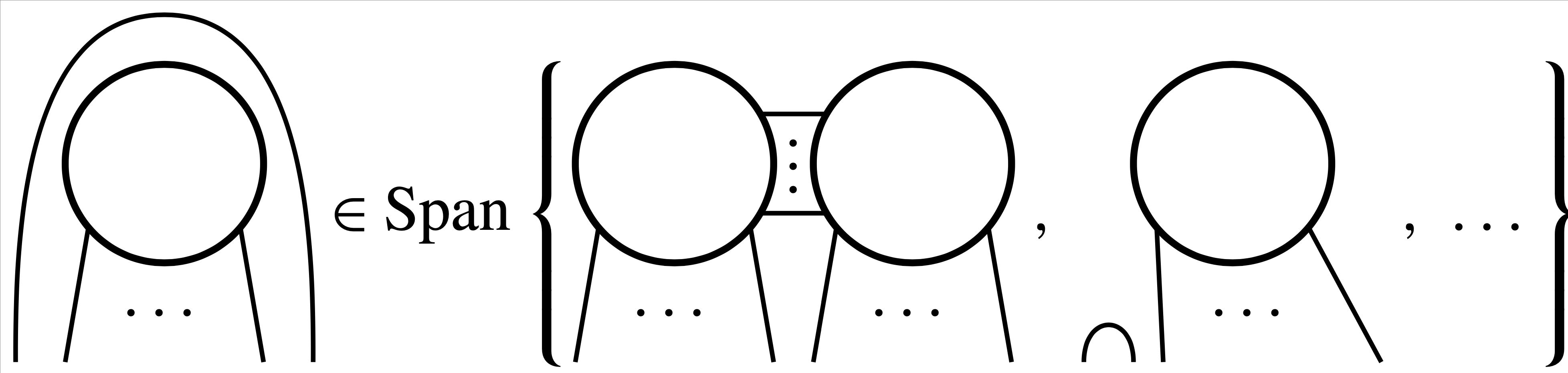
Ana­log­ous to the braid­ing re­la­tion, the ex­ten­ded Haagerup planar al­gebra has two braid­ing sub­sti­tute re­la­tions. The sim­pler of the two is of the form shown in Fig­ure 2. Again, the gen­er­at­or is a circle, and we have omit­ted the dis­tin­guished re­gions, the shad­ing, and the coef­fi­cients in the lin­ear com­bin­a­tion. We have also cheated with the el­lip­sis, which hides some terms that are dia­grams with no cop­ies of the gen­er­at­or.

Note that one of the terms on the right of the braid­ing sub­sti­tute re­la­tion has two cop­ies of the gen­er­at­or. However all gen­er­at­ors on the right are all closer to the top than the gen­er­at­or on the left. Thus, if we are will­ing to in­crease the num­ber of gen­er­at­ors in a dia­gram, we can move them all to the top.

Once we have all of the gen­er­at­ors at the top of a closed dia­gram, we can then start to de­crease the num­ber of gen­er­at­ors. If a gen­er­at­or is con­nec­ted to it­self by a “cup”, then the dia­gram is zero. If not, it is not hard to show there must be a pair of gen­er­at­ors that are joined by at least half of their strands. Such a pair can be sim­pli­fied by the quad­rat­ic re­la­tion. We can re­peat this pro­cess un­til there are no gen­er­at­ors.

The above eval­u­ation al­gorithm is called the jelly­fish al­gorithm, since the first stage is re­min­is­cent of jelly­fish float­ing to the top of a tank. The same al­gorithm has been used to con­struct oth­er sub­factors, for ex­ample in [e10]. Con­versely, it has been used to place re­stric­tions on the type of graphs that can be prin­cip­al graphs of sub­factors [e9].