Celebratio Mathematica

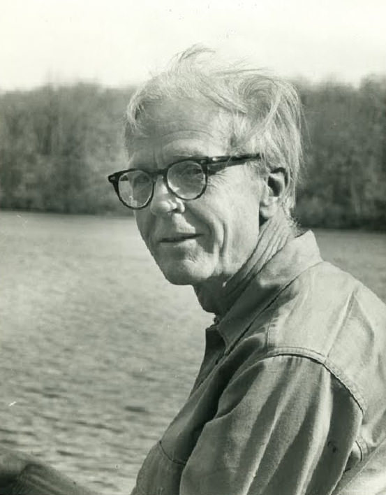
Hassler Whit­ney (March 23, 1907 – May 10, 1989) was one of the most ori­gin­al and in­flu­en­tial math­em­aticians of the twen­ti­eth cen­tury. He cre­ated the field of dif­fer­en­tial to­po­logy, and fa­mil­i­ar terms such as co­homo­logy, cobound­ary, cocycle, cup and cap products, co­homo­logy ring, are all his, stem­ming from his found­a­tion­al work in to­po­logy. He gave the defin­i­tion of dif­fer­en­ti­able man­i­fold still used today, and proved that any dif­fer­en­ti­able man­i­fold can be em­bed­ded in Eu­c­lidean space. His two em­bed­ding the­or­ems can jus­ti­fi­ably be called the grand­fath­ers of all em­bed­ding the­or­ems, and were the pre­curs­ors of hun­dreds of dif­fer­ent em­bed­ding the­or­ems seen today in geo­metry and al­gebra.

How did he do it? Whit­ney’s story is fas­cin­at­ing. His tale flies in the face of nearly everything con­ven­tion­al, and is one likely to sur­prise most people. He was not a math­em­at­ic­al prodigy who gobbled up text­books and knew more math than any of his school peers might ever hope to know. He re­min­isced later in life that “Thank­fully, I took al­most no math courses in either high school or col­lege…” He felt just plain lucky to have missed a hail of bul­lets. So again, how did he do it?

The an­swer seems to lie in how dis­tinct per­son­al­ity traits and early fam­ily in­flu­ences worked to­geth­er to form the per­son. We start our story by list­ing some of his per­son­al traits, as well as his main fam­ily in­flu­ences. We tell the big story it­self as a se­quence of vign­ettes — little snip­pets of things he did or things that happened to him. In the end, his un­usu­al story makes very good sense. In 1967, Deane Mont­gomery offered an in­ter­est­ing per­spect­ive on just how suc­cess­ful he was. (Mont­gomery con­trib­uted sig­ni­fic­antly to solv­ing Hil­bert’s fifth prob­lem, and for some years headed the School of Math­em­at­ics at the In­sti­tute for Ad­vanced Study in Prin­ceton.) “If you were to ask a good sampling of first-rate math­em­aticians to list the top 10 math­em­aticians in the world, Whit­ney would be on nearly every­one’s list.”

1. He was hap­pi­est when he was free, and be­came dis­tinctly un­happy when trapped in a situ­ation — so­cial or oth­er­wise — that was not to his lik­ing. He’d use wit, hu­mor or simply ab­rupt­ness to ex­tric­ate him­self from such a situ­ation. He hated be­ing en­slaved in any form. In high school and col­lege, he al­most nev­er read through a math­em­at­ics text or worked through the book’s prob­lems. In­stead, he would either make up his own prob­lems, or run across a prob­lem that caught his fancy, and then learn whatever math was needed to solve it.

2. When in­ter­ested in something, he could be end­lessly per­sist­ent.

3. When he was a young­ster, it was not at all clear that he would end up as a math­em­atician. He had a keen in­terest in the real world and in how things work. His early in­terests were in large part like those of an en­gin­eer or pos­sibly a phys­i­cist. He liked to run little sci­entif­ic ex­per­i­ments, and would build small ma­chines or some ap­par­at­us that he needed. His fa­vor­ite magazine was Pop­u­lar Sci­ence, and he would eagerly await the next is­sue. Ideas in it some­times in­spired new con­struc­tion pro­jects.

4. He nev­er liked grade school. He once said that if he didn’t have to con­tend with school, there would be enough time in the day to ac­com­plish what he really wanted to do.

5. He had a dis­tinctly con­trari­an streak, and of­ten sought the op­pos­ite to the con­ven­tion­al or un­writ­ten norm. As a kid, he learned to roller-skate back­wards al­most as well as he did for­wards. Later in life, when en­coun­ter­ing a the­or­em new to him, he would of­ten be­gin by try­ing to dis­prove it, look­ing every which way for some counter­example. After a peri­od of rough and tumble, he of­ten ended up with a depth of un­der­stand­ing that most people nev­er get by merely ac­cept­ing the the­or­em and fol­low­ing through its proof.

6. He was very con­crete in his ap­proach to math. He would find a spe­cif­ic ex­ample con­tain­ing the es­sen­tial dif­fi­culty, and would work with it un­til he thor­oughly un­der­stood it. He got crit­ic­al in­sights by work­ing with his ex­ample, and used those in­sights to ar­rive at new res­ults. After crack­ing the cent­ral nut in a new area, he would usu­ally leave it to oth­ers to gen­er­al­ize.

7. As for choos­ing a math­em­at­ics prob­lem to work on, it was al­ways something that, in his words, “would catch my fancy.” The prob­lem needed to be simple, ele­ment­ary, and one he could think about without hav­ing to get on top of a lot of ad­di­tion­al back­ground ma­ter­i­al. Find­ing just the right prob­lem, he learned, could be quite a chal­lenge.

8. He thought very geo­met­ric­ally, and drew lots of pic­tures. When it was time to write up a proof, he would re­for­mu­late the geo­metry in al­geb­ra­ic terms. But al­most al­ways his ori­gin­al in­spir­a­tion was geo­met­ric.

9. He end­lessly ana­lyzed things, and that was not just in math­em­at­ics. He did it in his oth­er pas­sions such as moun­tain climb­ing, com­pet­it­ive ice skat­ing and mu­sic.

10. His be­ha­vi­or in so­cial set­tings was highly con­di­tion­al. In the com­pany of moun­tain climbers or mu­si­cians, he could be charm­ing and witty. But those who knew him only in set­tings in which he couldn’t open up were more likely to de­scribe him as re­mote, de­tached, shy or ta­cit­urn. He sel­dom en­gaged in math­em­at­ic­al small talk. He would enter in­to a dis­cus­sion if it was rel­ev­ant to his cur­rent in­terests, but just shop talk? That al­most nev­er happened.

Our first story takes place soon after Hass learned how to mul­tiply num­bers in school. At one point it was men­tioned that whenev­er you mul­tiply a di­git by 9, the an­swer’s di­gits al­ways add up to 9. That is, in any of 9, 18, 27, 36, …, 81, the di­gits sum to 9. Hassler thought this was amaz­ing. Throughout his life, the key to un­leash­ing his sci­entif­ic en­ergy was to catch his fancy, and this re­mark­able fact did just that. He began to ex­per­i­ment with 9 times lar­ger num­bers, such as 9 times 10, 11, 12, 13, …, and sum­ming the di­gits un­til you get a single di­git still al­ways ended up giv­ing 9. He then tried really big num­bers, like 9 times 8,213, and the phe­nomen­on still held. He thought about this for a few days, and fi­nally con­vinced him­self that it was al­ways true, no mat­ter what big in­teger you mul­ti­plied by 9. He then tested the idea on mul­tiply­ing 1, 2, 3, … by 8 in­stead of 9, and found that in­stead of al­ways sum­ming to 9, the sum de­creased, get­ting a cycle that end­lessly re­peats: 8, 7, 6, 5, 4, 3, 2, 1, 9, 8, …. When mul­tiply­ing by 7, the se­quence went down by 2: 7, 5, 3, 1, 8, 6, 4, 2, 9, 7, …. Sym­met­ric­ally, if he mul­ti­plied by 10, which is 1 more than 9, the se­quence went up by 1: 1, 2, 3, …. Mul­tiply­ing by 11 (2 more than 9) gave a se­quence that in­creased by 2. Young Hassler was ex­cited by find­ing these reg­u­lar­it­ies, and he al­ways re­garded this as “my first little bit of math­em­at­ic­al re­search.”

Hassler moved to Switzer­land when he was 14, and spent two years there. His older sis­ter Car­oline had al­ways been ex­tremely sup­port­ive of Hass, and be­fore he moved she bought him a slide rule. In Switzer­land, he began to think about just how his slide rule per­forms its ma­gic. He learned about log­ar­ithms and some ba­sic ques­tions oc­cured to him. He un­der­stood why \( \log 1 \) is 0 and \( \log 10 \) is 1, but what about all the oth­er num­bers? He de­cided that find­ing \( \log 2 \) would be an ex­cel­lent pro­ject. Ac­cord­ing to the slide rule, it should be a little over \( 0.3 \), but how much over? Was there some way to find the value to a few decim­al places, to get a bet­ter an­swer than the slide rule could? He cooked up a plan of at­tack. If you mul­tiply 2 by it­self a bunch of times to get \( 2^n \), then the log­ar­ithm of that is \( n\log 2 \); if you mul­tiply 10 by it­self a bunch of times to get \( 10^m \), then that has a very simple log­ar­ithm, just \( m \). His scheme was this: keep on doub­ling 2 un­til you get 1 fol­lowed by \( m \) zer­os. At that point, \( n\log 2=m \), mean­ing that \( \log 2=m/n \). But as he doubled 2 over and over again, he soon real­ized that he could nev­er get the last di­git to be 0, since the last di­git end­lessly cycled 2, 4, 8, 6, 2, 4, 8, …. He cer­tainly didn’t know this ob­ser­va­tion es­sen­tially proves that \( \log 2 \) is ir­ra­tion­al! Nev­er­the­less, he hoped for a good ap­prox­im­a­tion. He got some­what close when \( n \) is 10, 20, 30, 40, but after filling up page upon page com­put­ing powers of 2 and al­ways miss­ing his goal of beat­ing the slide rule, he fi­nally gave up. He really tangled with this prob­lem, and gained a lot of re­spect for it.

In­creas­ingly things were hap­pen­ing in math that seemed mys­ter­i­ous to him. He was close to his older sis­ter Car­oline, and in a let­ter he muses, “What are the log­ar­ithms of neg­at­ive num­bers? Do they have any re­la­tion to ima­gin­ary num­bers? If they haven’t, I should think they would be pretty use­ful any­way.” Later, he be­gins to won­der why cer­tain graphs have “ex­cluded re­gions.” Even the parts to the left and right of a circle’s plot were ex­cluded, wer­en’t they? Was it be­cause of ima­gin­ary num­bers, again? He was meet­ing more and more mys­ter­ies, and his sub­con­scious was be­com­ing pre­pared for an­swers.

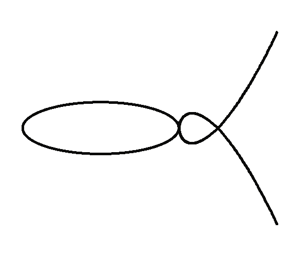
It de­lighted Hass to see that ab­stract com­bin­a­tions of sym­bols as in poly­no­mi­als could be pic­tured geo­met­ric­ally. He would make up poly­no­mi­als and use his slide rule to com­pute points on the graph, then con­nect the points to get the rest of the graph. When he stumbled upon \( y=1/x \), something weird happened — the graph (a hy­per­bola) broke up in­to two parts. Could he make up graphs that broke up in­to three parts? four? five? In a long let­ter to Car­oline writ­ten over a few days from Switzer­land, he chron­icles his pro­gress in this, and you can see his un­der­stand­ing be­gin­ning to grow. A little later he stumbles upon a dif­fer­ent idea: re­place \( y \) by \( y^2 \). Now, sud­denly, the graph is sym­met­ric about the \( x \)-ax­is. In ex­plor­ing this idea, he happened to plot \( y^2=x^3+x^2 \). To his com­plete sur­prise, he found it looked like a bug’s head to­geth­er with two an­ten­nae com­ing out! He’d been fas­cin­ated by bugs and crawly things ever since he’d been a small boy, and now an equa­tion could rep­lic­ate some of that. He was on a roll, and wanted some way to give the bug a body. He even­tu­ally real­ized that if you plot \( f(x,y) = 0 \) and \( g(x,y) = 0 \), then the uni­on of the two plots is giv­en by the plot of \( fg = 0 \). So by ap­pro­pri­ately mul­tiply­ing equa­tions, he was able to add an el­lipse-shaped body to the head. Us­ing this same idea, he could add small circles or el­lipses to rep­res­ent dots of the kind you see on a lady­bug.

Hass re­turned to the States in 1923, and had just one more year be­fore en­ter­ing col­lege at Yale. His hanker­ing for meas­ur­ing things now ex­ten­ded to find­ing lengths of vari­ous curves. By this time he knew that cal­cu­lus could help in find­ing lengths, areas and volumes. He owned a cal­cu­lus book, but had not the slight­est in­clin­a­tion to sit down and read it, or go through ex­er­cises in it. For him, the book was a re­source, a hand­book that he might use to help solve prob­lems that in­ter­ested him. One such prob­lem he thought about was this: “If an ant crawls along one arch of the sine curve, how far has it trav­elled?” After set­ting up the cor­rect in­teg­ral, he found that nowhere in the table of in­teg­rals at the back of the book was there any­thing that could solve the prob­lem for him. He ended up with an ap­prox­im­a­tion, es­sen­tially get­ting the lengths of small pieces of the curve and adding them up.

Ex­per­i­ences of this sort made him quite a bit wiser than stu­dents who would read about arc length, do the book’s prob­lems, get the right an­swers, take a test and re­ceive an “A”. “They come away think­ing they can find arc lengths! Gee, the book care­fully chooses prob­lems so the stu­dents see only those rare ex­amples where things work out nicely. They can go the rest of their life hav­ing a totally un­real­ist­ic view.”

In 1928, after four years at Yale, Hass gradu­ated as a phys­ics ma­jor. He took an ad­di­tion­al year there to earn a second Bach­el­or’s de­gree, this time in mu­sic. But he’d made his ca­reer choice — the­or­et­ic­al phys­ics. Be­fore com­plet­ing his mu­sic de­gree, he de­cided to spend three weeks in the sum­mer of 1928 to breathe in and ab­sorb the at­mo­sphere of phys­ics and math­em­at­ics in Göt­tin­gen, Ger­many. As a sopho­more, he had taken a gradu­ate course en­titled “Gen­er­al the­ory of math­em­at­ic­al phys­ics,” and had taken vo­lu­min­ous notes filling up five bind­ers. He took these with him, since it seemed that re­fa­mil­i­ar­iz­ing him­self with them would give him a run­ning start at Har­vard. He felt com­fort­able in Göt­tin­gen, and im­me­di­ately made friends with Dir­ac. The two shared time puzz­ling over little num­ber-the­ory prob­lems.

After a week of en­joy­ing him­self, it was time to blitz through those five bind­ers. Day 1: he was as­ton­ished to dis­cov­er he had for­got­ten nearly everything in the notes. Day 2: things still wer­en’t com­ing back to him. Day 3: ditto, but he still had nearly two weeks. After ad­di­tion­al days of strug­gling, a hor­rible real­ity was be­gin­ning to emerge: in phys­ics, you have to re­mem­ber stuff, and it seemed he ac­tu­ally had no head for that. Halfway through the second week of this, he es­sen­tially threw up his hands in des­pair and asked him­self, “What am I gonna do?”

He def­in­itely wasn’t en­joy­ing this, and he began tak­ing ser­i­ous stock of him­self. What were his stel­lar mo­ments? his worst mo­ments? His biggest high points at Yale nev­er oc­curred in phys­ics, but rather in math­em­at­ics. For ex­ample, in one class taught by the le­gendary James Pier­pont, the fam­ous man singled out Hass: “Mr. Whit­ney says he ‘just’ learns math on his own! How did Riemann learn math­em­at­ics? How did Wei­er­strass do it? Just like Whit­ney here, on their own! That’s the very best way!” An­oth­er time, Hass had turned in an es­pe­cially in­geni­ous ex­ample of an every­where dis­con­tinu­ous func­tion. Pier­pont held it up as an ex­ample of “pure geni­us.” Hassler’s worst mo­ments were in re­quired his­tory courses — for years he ac­tu­ally had night­mares about not be­ing able to re­mem­ber things for an up­com­ing his­tory ex­am. And what did he really love to do? A fel­low stu­dent at Yale had once men­tioned the four-col­or con­jec­ture, and it fas­cin­ated him. He greatly en­joyed think­ing about the prob­lem in odd mo­ments. To him, it was re­cre­ation. Plus, no one had ever solved it, so there was a car­rot dangling in front of him. Look­ing back on what he was good at and what he en­joyed, it seemed that think­ing about math­em­at­ics prob­lems checked both boxes.

After per­haps the most un­com­fort­able few days in his life, Hassler made a de­cision: his life would be in math­em­at­ics, not phys­ics. To­ward the end of his ca­reer he re­min­isced, “I have al­ways re­gret­ted my quandary, but nev­er re­gret­ted my de­cision.”

Once at Har­vard, he im­me­di­ately switched to math­em­at­ics and began think­ing about the four-col­or prob­lem. He put the prob­lem in­to a dif­fer­ent form: he re­placed each colored coun­try by a colored cap­it­al, and, if two coun­tries shared a com­mon bound­ary, he drew a road con­nect­ing their cap­it­als. Es­sen­tially, he was think­ing about colored graphs. The goal was that, by us­ing just four col­ors, you can col­or the cap­it­als so that the road from one coun­try to a neigh­bor­ing coun­try would al­ways con­nect dif­fer­ently colored cap­it­als. This area had really caught his fancy, and al­though he en­rolled in courses and at­ten­ded them, his real ef­fort was spent think­ing in an area that had cap­tured his ima­gin­a­tion.

Hass worked by him­self for many weeks on the prob­lem, mak­ing count­less draw­ings with cap­it­als rep­res­en­ted by colored points. From all these draw­ings, he used his nat­ur­al abil­ity to make con­jec­tures, test them, and ar­rive at some res­ults that ap­peared to be new. Of course his main aim in go­ing to gradu­ate school was to get a Ph.D., and he needed an ad­visor for that. He asked around and soon learned that George Birk­hoff fit the bill. Birk­hoff had done some work on the four-col­or con­jec­ture, so Hass paid him a vis­it, and showed him the res­ults he had ob­tained.

Birk­hoff im­me­di­ately re­cog­nized that Hassler, com­pletely on his own, had come up with some in­sights that Birk­hoff him­self had totally missed. Birk­hoff in turn shared with Hass some of his own in­sights he’d got­ten earli­er, and the two fell in­to a sym­bi­ot­ic friend­ship. Hass says in a let­ter, “Birk­hoff, more than any­one else in the world, thinks the same way I do!” Every so of­ten, Hass would drop by and show Birk­hoff his latest res­ults. After a while, Hassler felt he’d pro­gressed far enough on the prob­lem to war­rant writ­ing it up as his thes­is. Birk­hoff went over the top with en­thu­si­asm: “With what the two of us have here, I es­tim­ate there’s a one-in-five chance that we’ll prove the four-col­or con­jec­ture!” Hass was more cau­tious, and felt a proof was at least 50 years away. He wasn’t far off — Ap­pel and Haken an­nounced their com­puter proof in 1976, just 46 years after Whit­ney’s guess­tim­ate.

Birk­hoff gave Hass some ex­tremely help­ful ad­vice: “Write up the high points of your work right away, and sub­mit it to the Pro­ceed­ings of the Na­tion­al Academy of Sci­ences. Neither of us would want someone to an­ti­cip­ate your res­ults. Then, after that, write up a more com­plete ac­count with full proofs, and sub­mit that to the An­nals.” Hass had his work cut out for him, but by fol­low­ing his in­ner ur­gings and ar­riv­ing at new res­ults about a prob­lem he loved think­ing about, he ended up with three pa­pers [2], [3], [1] in those ex­cel­lent journ­als. Earli­er, Birk­hoff had got­ten him an In­struct­or­ship at Har­vard, pay­ing \$3,000 for the year. Now, he wrote a let­ter “that couldn’t be stronger,” re­com­mend­ing Hass to the po­s­i­tion of As­sist­ant Pro­fess­or at Har­vard for the three years 1934–36, with wages of \$4,000, \$4,300 and \$4,600 — not bad num­bers in those days. Hassler’s ini­tial teach­ing sched­ule was not es­pe­cially de­mand­ing, con­sist­ing of a course on cal­cu­lus and one on dif­fer­en­tial equa­tions. He was giv­en plenty of time to think math­em­at­ics.

Des­pite his love for and pro­gress on the four-col­or prob­lem, Hass nev­er in­ten­ded to spend his en­tire ca­reer on it. In him was a need to do something he thought was “real math­em­at­ics,” in the sense of more tra­di­tion­al ana­lys­is — something that would in­volve dif­fer­en­ti­able func­tions. After all, he had spent years in phys­ics work­ing with poly­no­mi­als, tri­go­no­met­ric and ex­po­nen­tial func­tions, and they were his friends. He began to keep an eye out for some prob­lem in­volving dif­fer­en­ti­able func­tions that would catch his fancy. It had to be ele­ment­ary, simply stated, re­quire little ex­tra back­ground to make pro­gress, and in­volve dif­fer­en­ti­able func­tions in some way.

His quarry proved sur­pris­ingly elu­sive, but after a few months he fi­nally stumbled upon what he wanted: an eight-page art­icle writ­ten by Wil­li­am Why­burn that gen­er­al­ized the Tiet­ze ex­ten­sion the­or­em for con­tinu­ous func­tions, to cer­tain dif­fer­en­ti­able ones. (In Eu­c­lidean \( n \)-space \( \mathbb E^n \), the Tiet­ze the­or­em says that a func­tion con­tinu­ous on a closed set in \( \mathbb E^n \) has a con­tinu­ous ex­ten­sion to all of \( \mathbb E^n \).) This art­icle, “Non-isol­ated crit­ic­al points of func­tions” [e1] which ap­peared in the Bul­let­in of the AMS 35 (1929), pp. 701–708, in­spired Hassler to ask two big, cent­ral ques­tions: (1) If in some sense a func­tion is \( n \)-times dif­fer­en­ti­able on any closed set of \( \mathbb E^n \), can it be ex­ten­ded to an \( n \)-times dif­fer­en­ti­able func­tion on all of \( \mathbb E^n \)? (2) If the func­tion is ana­lyt­ic on the closed set, is there an ana­lyt­ic ex­ten­sion to \( \mathbb E^n \)? The an­swers would be sig­ni­fic­ant no mat­ter how they turned out.

In what can now be called clas­sic Whit­ney style, he con­sidered lots of ex­amples, drew many pic­tures, con­sidered many ways of cre­at­ing ex­ten­sions, and through per­sist­ence fi­nally got loc­al ex­ten­sions to match up prop­erly. It was a break­through for him, and a break­through for math­em­at­ics. He ad­mits, “It wasn’t that easy,” but in 1934 his 27-page art­icle [4] ap­peared in the Trans­ac­tions of the AMS. His next four pa­pers also came out in 1934, and were all in this genre, one ap­pear­ing in the Bul­let­in of the AMS, one in the Trans­ac­tions and two in the An­nals of Math­em­at­ics. The year 1934 was a good one for the 27-year-old.

By 1930 there were sev­er­al com­pet­ing defin­i­tions of a dif­fer­en­ti­able (or smooth) man­i­fold, and in 1932 Veblen and White­head had de­vised an ab­stract defin­i­tion that uni­fied the dif­fer­ent ap­proaches and had the aim of sup­ply­ing dif­fer­en­tial geo­metry with a more sol­id and up­dated found­a­tion. Whit­ney was al­ways one for con­crete­ness, and he, as well as oth­ers, wondered if the ab­stract defin­i­tion was really ne­ces­sary. Did it ac­tu­ally in­clude new ob­jects, ob­jects oth­er than those man­i­folds already sit­ting in some Eu­c­lidean space? If not, then the ab­stract concept could simply be dis­carded, mean­ing any dif­fer­en­ti­able man­i­fold could be defined in some Eu­c­lidean space of high-enough di­men­sion, us­ing patches glued to­geth­er by dif­feo­morph­isms on their over­lap­ping parts.

As for­tune would have it, Hassler’s work on ex­tend­ing dif­fer­en­ti­able func­tions provided some es­sen­tial tools needed in an­swer­ing the ques­tion. In 1936, he was able to prove [5] that any \( n \)-di­men­sion­al com­pact con­nec­ted dif­fer­en­ti­able man­i­fold, in the sense of Veblen and White­head, could in fact be real­ized as a sub­set of a Eu­c­lidean space of di­men­sion \( 2n+1 \). Eight years later [7], us­ing meth­ods from al­geb­ra­ic to­po­logy, he was able to prove a stronger form, re­du­cing the \( 2n+1 \) to \( 2n \).

A simple case of the stronger the­or­em would be a fancy knot­ted loop in a real space of any di­men­sion, the loop be­ing dif­fer­en­ti­ably em­bed­ded there. In this case \( n=1 \), so the the­or­em guar­an­tees a dif­feo­morph­ism between it and, say, a circle in \( \mathbb E^{n} \), which is the real plane.

For oth­er ex­amples, con­sider fa­mil­i­ar man­i­folds such as the Klein bottle or the real pro­ject­ive plane. The Klein bottle can be ob­tained by cut­ting a tor­us to make a long hose, and then re­con­nect­ing the two cir­cu­lar, freshly-cut bound­ar­ies so their ori­ent­a­tions are op­pos­ite. A real pro­ject­ive plane can be con­struc­ted by sew­ing to­geth­er a Möbi­us strip and a disk along their cir­cu­lar bound­ary. Both the Klein bottle and the real pro­ject­ive plane are \( n \)-man­i­folds with \( n=2 \), and neither of them can be real­ized in or­din­ary 3-space without self-in­ter­sec­tions. Whit­ney’s stronger em­bed­ding the­or­em guar­an­tees that each of them can ex­ist in \( \mathbb E^{2n}=\mathbb E^4 \) as a smooth, and there­fore non-self-in­ter­sect­ing, man­i­fold. Ac­tu­ally, there’s what might be called a “poor man’s ver­sion” of an em­bed­ding — an im­mer­sion — that per­mits well-be­haved sin­gu­lar­it­ies, and in this case Whit­ney showed the di­men­sion can be lowered to \( 2n-1 \). For ex­ample, a glass mod­el of the Klein bottle in or­din­ary 3-space \( \mathbb E^3=\mathbb E^{2\cdot2-1} \) rep­res­ents an im­mer­sion of the Klein bottle in 3-space. The circle where the handle in­ter­sects the main part of the bottle is a trans­verse in­ter­sec­tion, which is suf­fi­ciently nice.

An es­sen­tial step in Whit­ney’s ori­gin­al \( 2n \) the­or­em is the fam­ous “Whit­ney trick.” A de­scrip­tion of this by Ro­bi­on Kirby can be read here.

Whit­ney’s em­bed­ding the­or­em changed the land­scape of man­i­fold the­ory. Since any man­i­fold can now be put in some Eu­c­lidean space, the man­i­fold in­her­its a met­ric from that sur­round­ing space. At any point \( P \) of the man­i­fold, it makes sense to talk about a point \( Q \) close to \( P \), and there­fore also the line through \( P \) and \( Q \), as well as the lim­it line as \( Q \) ap­proaches \( P \), and there­fore the tan­gent space to the man­i­fold at any one of its points \( P \). Since the am­bi­ent space is Eu­c­lidean, there’s also the vec­tor space of all vec­tors nor­mal to the man­i­fold at that point \( P \). This point­wise or­tho­gon­al de­com­pos­i­tion was to play an im­port­ant role in Whit­ney’s sub­sequent re­search.

The met­ric also means we can define with­in the tan­gent space such things as a sphere about \( P \). The same can be done with­in the nor­mal space. Do­ing this at each point of the man­i­fold so that the uni­on is smooth yields tan­gent sphere bundles and nor­mal sphere bundles. One can also form products at each point; these are loc­al products. For ex­ample, at each point of a loop in 3-space, one can con­struct a unit in­ter­val per­pen­dic­u­lar to the loop, the in­ter­vals vary­ing smoothly along the loop base space. Glob­ally, there are two dis­tinct to­po­lo­gic­al ways to do this, giv­ing on the one hand a to­po­lo­gic­al cyl­in­der, and on the oth­er a Möbi­us strip. One can as­sign a de­gree of twist­ing or tor­sion to each pos­sib­il­ity, 0 to the cyl­in­der and 1 to the Möbi­us strip. This can be re­cast in­to the lan­guage of spheres: an in­ter­val is a 1-ball, and its two-point bound­ary is a 0-sphere. If the strip is giv­en an even num­ber of half-twists, the 0-spheres form two to­po­lo­gic­al loops, where­as an odd num­ber yields just a single loop. 0 and 1 can nat­ur­ally be re­garded as the group ele­ments of the in­tegers mod 2.

It seemed likely that this phe­nomen­on also oc­curs in high­er di­men­sions, and that there ought to be a way to sim­il­arly quanti­fy the be­ha­vi­or. Even­tu­ally, a vec­tor over the in­tegers mod 2 cap­tured the tor­sion in­form­a­tion with­in a more gen­er­al sphere bundle — es­sen­tially a Stiefel–Whit­ney char­ac­ter­ist­ic class. All this is very much con­nec­ted to the ho­mo­logy of sphere bundles. Soon, Whit­ney found a way to ex­press things in a more power­ful and nat­ur­al way us­ing co­homo­logy.

Du­al­ity played a big part in Whit­ney’s math­em­at­ic­al re­search. Even in his first mus­ings about the four-col­or prob­lem, he trans­formed a geo­graph­ic­al map — a planar graph — in­to its dual, and mostly worked with that. A map nat­ur­ally di­vides the plane in­to a sim­pli­cial com­plex, and as­so­ci­ated to each \( r \)-sim­plex is a \( (2-r) \)–sim­plex: a coun­try is a 2-sim­plex, and its as­so­ci­ated dual \( (2-2)=0\, \)-sim­plex (a point) is its cap­it­al. The bound­ary between two coun­tries is a 1-sim­plex, and its dual is a \( (2-1)=1\, \)–sim­plex (a road) cross­ing the bound­ary trans­vers­ally. A ver­tex of the ori­gin­al graph du­al­izes to the 2-sim­plex in the new graph that con­tains that ver­tex. (This idea is fa­mil­i­ar to elec­tric­al en­gin­eers, who of­ten form the dual of a planar elec­tric­al cir­cuit to sim­pli­fy solv­ing a prob­lem.)

He was able to gen­er­al­ize this key idea to sim­pli­cial com­plexes of any di­men­sion \( n \), in which as­so­ci­ated to any \( r \)-sim­plex is a dual \( (n-r) \)–sim­plex. Im­port­antly, the ho­mo­logy of the ori­gin­al com­plex is es­sen­tially the same as the co­homo­logy of the dual com­plex, and now Whit­ney massively pushed for­ward ex­ist­ing ho­mo­lo­gic­al fron­ti­ers. A few years earli­er, Poin­caré’s Betti num­bers had been giv­en a group struc­ture by Emmy No­eth­er, and now Whit­ney was able to define a product (the cup product) so that the dir­ect sum of co­homo­logy groups be­came a co­homo­logy ring. To­po­lo­gic­al in­vari­ants of a man­i­fold could now be ex­pressed in a more nat­ur­al way us­ing the man­i­fold’s co­homo­logy ring.

In 1935, Whit­ney at­ten­ded the In­ter­na­tion­al Con­fer­ence in To­po­logy held in Mo­scow and learned that J. W. Al­ex­an­der and A. N. Kolmogoroff had in­de­pend­ently pro­posed a way to form products of sim­pli­cial com­plexes. This greatly in­ter­ested Whit­ney, but he felt something wasn’t quite right about their defin­i­tion. To­geth­er with E. Čech, Whit­ney fixed things, thus open­ing up the way for geo­met­ric op­er­a­tions on bundles. With the defin­i­tions and tools that Whit­ney now had, he was even­tu­ally able to de­scribe char­ac­ter­ist­ic classes of the Whit­ney sum of two bundles — a cent­ral res­ult now known as the Whit­ney Product the­or­em.

In 1952, at age 45, Hass ac­cep­ted an of­fer from the In­sti­tute for Ad­vanced Study in Prin­ceton to join the fac­ulty “without term” — mean­ing he was in­vited to be­come a per­man­ent mem­ber. There were some big pro­jects that he had al­ways wanted to work on, and this piece of good news would al­low him to pur­sue these without hav­ing to pre­pare lec­tures or grade pa­pers.

One of these pro­jects was to ex­pand in­to a book his well-re­ceived 41-page ac­count of his work on sphere bundles [6], which ap­peared in Lec­tures in To­po­logy, Univ. of Michigan Press, 1941. To pre­pare a found­a­tion for the book, he wrote the book Geo­met­ric in­teg­ra­tion the­ory [9], which ad­dresses is­sues of in­teg­ra­tion on man­i­folds hav­ing sin­gu­lar­it­ies. Al­though the book is full of ori­gin­al geo­met­ric ideas, he nev­er­the­less felt there re­mained non­trivi­al dif­fi­culties in ar­riv­ing at a sat­is­fact­ory geo­met­ric found­a­tion for the to­po­lo­gic­al side of his pro­posed book on sphere bundles. To his im­mense re­lief, Nor­man Steen­rod even­tu­ally came out with an out­stand­ing book on fiber bundles. Hass said, “Steen­rod did a far bet­ter job than I could pos­sibly have done.”

At the In­sti­tute, his first big pa­per was “Map­pings of the plane in­to the plane” [8], which ap­peared in the An­nals in 1955, (vol. 62, pp. 374–410). This pa­per can be looked at as an early har­binger of chaos the­ory, since it was a start­ing point for René Thom’s cata­strophe the­ory which, in turn, de­scribes a center­piece of chaos the­ory — bi­furc­a­tions.

In an­oth­er dir­ec­tion, he had proved much earli­er that \( n \)-di­men­sion­al man­i­folds could be im­mersed in \( (2n-1) \)-space, the im­mer­sion per­mit­ting cer­tain sin­gu­lar­it­ies. He real­ized that as­sum­ing man­i­folds were al­ways smooth was too re­stric­ted — lots of nat­ur­ally oc­cur­ring sets had sin­gu­lar­it­ies as part and par­cel of their nature, al­geb­ra­ic vari­et­ies be­ing one ubi­quit­ous ex­ample. He saw that such sets of­ten nat­ur­ally break up in­to sim­pli­cial com­plexes. One simple ex­ample harkens all the way back to his teen­age mus­ings about graph­ing poly­no­mi­als — the real “al­pha curve” defined by \( y^2=x^3+x^2 \) that looked like a bug’s head with two an­ten­nae com­ing out. The part of this curve cor­res­pond­ing to nonzero \( x \) nat­ur­ally falls in­to three parts: the two an­ten­nae and the head — each of these pieces is a to­po­lo­gic­al open 1-cell. The sin­gu­lar­ity at the ori­gin nat­ur­ally defines a 0-cell.

This idea ex­tends eas­ily to high­er di­men­sions, as well as to the com­plex set­ting. Hass wrote up his ideas, even­tu­ally ap­pear­ing as a 1965 An­nals art­icle, “Tan­gents to an ana­lyt­ic vari­ety” [10]. Hass wanted to lay the found­a­tions for a strat­i­fic­a­tion the­ory at the ana­lyt­ic-vari­ety level, and as a back­ground for this he wrote his second and fi­nal book, Com­plex ana­lyt­ic vari­et­ies [11]. Whit­ney was far-sighted and sensed that strat­i­fied man­i­folds would play an im­port­ant role in the fu­ture. In 1994 the lead­ing dif­fer­en­tial geo­met­er S. S. Chern wrote that he felt strat­i­fied man­i­folds would even­tu­ally be the main ob­jects of study in dif­fer­en­tial geo­metry. “They already play an im­port­ant role in MacPh­er­son’s the­ory of per­verse sheaves,” he said.

Throughout his life, Hass showed little in­terest in hob­bies. What he had were pas­sions: he was pas­sion­ate about math, mu­sic, moun­tain­eer­ing and ice skat­ing.

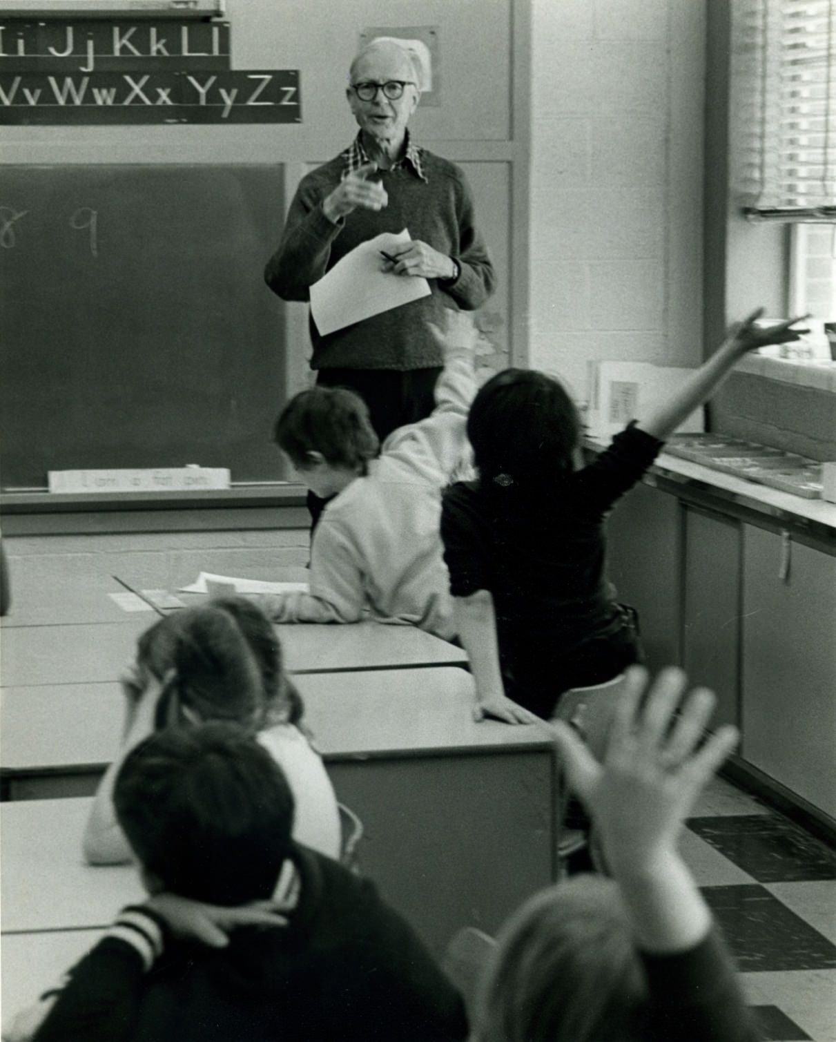
Around the age of 60, after he had mostly com­pleted his con­tri­bu­tions to math­em­at­ic­al re­search, he happened to pay a classroom vis­it to see how his two daugh­ters, Sally and Emily, were be­ing taught math. He was ap­palled by what he saw: ele­ment­ary school kids were be­ing forced away from their nat­ur­al in­stincts of reas­on­ing and learn­ing from ex­per­i­ence — the mode that served them so well in learn­ing an in­cred­ible amount in their preschool years — and made to “do” math ac­cord­ing to a new and strange classroom re­gi­men, where they were be­ing taught to use their pen­cils rather than their heads. He wondered, “What would have happened to me, had I been forced through such a sys­tem?” He did some re­search and found that the na­tion­al situ­ation was even worse than he had guessed. For ex­ample in one large study, 9-year-olds were asked to find how much fence was needed to en­close a \( 10^{\prime} \) by \( 6^{\prime} \) rect­angle, and a pi­ti­ful 9% of the kids got the right an­swer. “Heav­ens, if their mom or dad were plant­ing a garden in that shape and asked their little one to see how much fen­cing was needed to go around to keep the an­im­als out, one’s nat­ur­al in­stincts could well have led to the right an­swer. But in a classroom? It was all al­gorithms, com­pu­ta­tion, timed tests, …” Such real­iz­a­tions planted the seeds for his last great call­ing and pas­sion in life: chan­ging the way young kids were ex­posed to and taught math. He saw it as a chal­lenge of the highest im­port­ance. Al­ways pro­act­ive, Hass spent his re­main­ing years trav­el­ing with­in and out­side the States, teach­ing math in ele­ment­ary schools and run­ning work­shops with the aim of im­prov­ing math­em­at­ics edu­ca­tion.

Hassler suffered a stroke at age 82 in Prin­ceton (not Switzer­land, as some in­ter­net sources say), and died two weeks later. He had ap­par­ently been in good health, and phys­i­cians ul­ti­mately placed the blame on treat­ments for pro­state can­cer. A fel­low climber placed his ashes atop Mt. Dent Blanche in Switzer­land.

It is a pleas­ure to ac­know­ledge the help and in­put from Hassler’s chil­dren: James, Car­ol, Molly, Sally and Emily — as well as his wid­ow Bar­bara Os­ter­man. They have shared with me in­valu­able re­min­is­cences, and most of the pho­tos would have been im­possible to ob­tain without their help. In ad­di­tion, they have cri­tiqued vari­ous drafts of the bio­graphy. My great thanks to them all.