by Laurent Siebenmann
French to English translation by Min Hoon Kim and Mark Powell
Introduction
At the end of the summer of 1981, in San Diego, M. Freedman proved that every smooth homotopy 4-sphere \( M^4 \) is homeomorphic to \( S^4 \). Our main goal is to give an exposition of his proof. In this paper, every manifold will be metrisable and finite dimensional. We do not know yet whether such an \( M^4 \) is always diffeomorphic to \( S^4 \). On the other hand, Freedman proved that every topological homotopy 4-sphere \( M^4 \) (without any given smooth structure) is actually homeomorphic to \( S^4 \) (see below).
H. Poincaré conjectured that every smooth, homotopy \( n \)-sphere \( M^n \) is diffeomorphic to \( S^n \). The first nontrivial case, dimension 3, remains open (in 1982) despite the efforts of countless mathematicians. An amusing detail is that the counterexample of J. H. C. Whitehead [e1] to his own erroneous proof of this conjecture will play a large role in this lecture (see Section 2).
J. Milnor [e4] discovered smooth manifolds \( M^7 \) which are homeomorphic to \( S^7 \) but not diffeomorphic to \( S^7 \) (such exotic spheres exist in dimension \( \geq 7 \) [e13]). Therefore the above Poincaré conjecture has to be revised for dimension \( \geq 7 \). S. Smale [e9] established his theory of handles to prove that every smooth homotopy \( n \)-sphere is homeomorphic to \( S^n \) for \( n\geq 6 \). His technical result, the \( h \)-cobordism theorem (see below) is more precise. Combining this with surgery techniques of Kervaire–Milnor [e13] establishes the \( n=5 \) and 6 cases of the above Poincaré conjecture. M. Newman adapted the engulfing method of J. Stallings to prove the purely topological version, that is, every topological homotopy \( n \)-sphere is homeomorphic to \( S^n \) if \( n\geq 5 \). (Smale’s surgery method has also been adapted to the topological category [e29].) In summary, the Poincaré conjecture is essentially resolved in dimension \( \geq 5 \), is not resolved in dimension 3, and is partially resolved in dimension 4.
We sketch a proof of Freedman’s theorem which implies the topological classification of smooth, simply connected closed 4-manifolds and many other results of fundamental importance. Let \( V \) and \( V^{\prime} \) be two such manifolds. Suppose that there is an isomorphism \[ \Theta : H_2(V)\to H_2(V^{\prime}) \]
which preserves the intersection forms. (Note that \( V \) is a homotopy 4-sphere if and only if \( H_2(V)=0 \).)
Proof. It is not difficult to realise \( \Theta \) by a homotopy equivalence \( g : V\to V^{\prime} \) [e25]. Surgery theory [e14], [e21] gives a compact 5-manifold \( W \) with boundary \( \partial W=V\sqcup -V^{\prime} \) such that the inclusions \( V\to W \) and \( V^{\prime}\to W \) are homotopy equivalences and such that the restriction \( r|_V : V\to V^{\prime} \) of the retraction \( r : W\to V^{\prime} \) is homotopic to \( g \). The compact triad \( (W;V,V^{\prime}) \) is called an \( h \)-cobordism. Smale’s theory of handles tries to improve a Morse function \[ f : (W;V,V^{\prime})\to ([0,1];0,1) \]
to obtain a situation where \( f \) has no critical points, that is, \( f \) is a smooth submersion. Then \( W \) is a fibre bundle over \( [0,1] \) (a remark of Ehresmann) and hence \( W \) is diffeomorphic to \( V\times [0,1] \). We are going to find a topological submersion \( f \) which shows that \( W \) is a topological fibration on \( I \) (see [e23], Section 6) so that \( W \) is homeomorphic to \( V\times [0,1] \). ◻
In particular, we will prove the simply connected, topological 5-dimensional \( h \)-cobordism theorem.
For \( n\geq 6 \), instead of 5, Smale’s \( h \)-cobordism theorem gives the stronger conclusion that \( W \) is diffeomorphic to \( V\times [0,1] \). In dimension 5, his methods apply, but leaving to prove that \( W \) is diffeomorphic to \( V\times [0,1] \). The following problem is not yet resolved.
be
two families of disjointly embedded 2-spheres in a simply connected
4-manifold \( M \) (in fact \( f^{-1}(\text{a point}) \)) in such a way that the
homological intersection number \( S_i\cdot S_j^{\prime}=\pm \delta_{i,j} \). Can one
reduce \( S\cap S^{\prime} \) to \( k \) points of intersection (smooth and transverse)
by a smooth isotopy of \( S \) in \( M \)?
Similarly, to obtain the fact that \( W \) is homeomorphic to \( V\times [0,1] \), we claim (see [e15] and [e29], Essay III) that it suffices to solve the following problem.
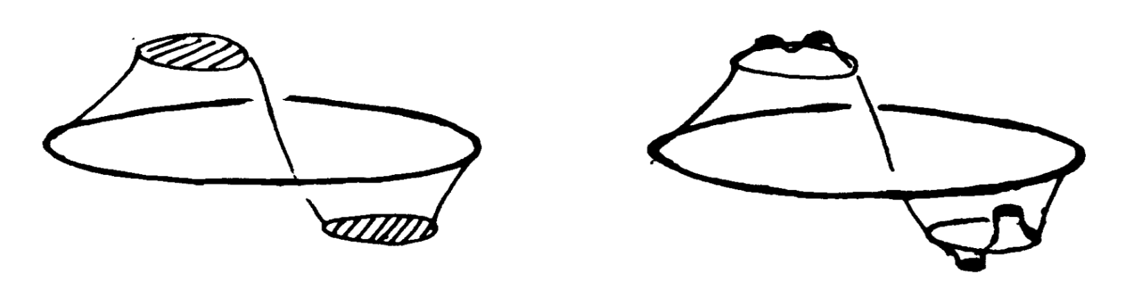
Whitney introduced a natural method for solving these problems. In the model \( (\mathbb{R}^2;A,A^{\prime}) \), (this is a straight line \( A \) cutting a parabola \( A^{\prime} \) in two points), we can disengage \( A \) from \( A^{\prime} \) by a smooth isotopy with compact support (that is, fixing a neighbourhood of \( \infty \)). One eliminates thus the two intersection points. We deduce that in the stabilised Whitney model, \[ (\mathbb{R}^4;A_+^{\vphantom{^{\prime}}},A_+^{\prime})=(\mathbb{R}^2\times \mathbb{R}^2;A\times 0\times \mathbb{R}, A^{\prime}\times \mathbb{R}\times0), \]
there is an isotopy with compact support that makes the plane \( A_+^{\vphantom{^{\prime}}} \) disjoint from the plane \( A_+^{\prime} \), deleting the two transverse intersection points between \( A_+^{\vphantom{^{\prime}}} \) and \( A_+^{\prime} \).
We call a smooth (resp. topological) Whitney process, a smooth embedding (resp. a topological embedding) of a disjoint union of copies of the model \( (\mathbb{R}^4;A_+^{\vphantom{^{\prime}}},A_+^{\prime}) \), whose image contains \( S\cap S^{\prime}\smallsetminus (k \text{ points}) \). Such a procedure would clearly give the demanded isotopy to resolve the remaining smooth problem (respectively, the remaining topological problem).
The first step of the proof (1973–1976) is due to A. Casson. Let \( B \) be a smooth, compact 2-disc in the boundary component of \( \mathbb{R}^2\smallsetminus A\cup A^{\prime} \). The product \( B\times \mathbb{R}^2 \) is an open, embedded 2-handle (as a closed submanifold) in the Whitney model, and disjoint from \( A_+^{\vphantom{^{\prime}}}\cup A_+^{\prime} \). In \( B\times \mathbb{R}^2 \), Casson constructed certain open sets \( H=B\times \mathbb{R}^2\smallsetminus \Omega \) with boundary \( \partial H=\partial B\times \mathbb{R}^2 \), that we call open Casson handles. (See Section 2 for the precise definition). We are again unable (in February 1982) to decide whether \( H \) is diffeomorphic to \( B\times \mathbb{R}^2 \) or not. Replacing \( B\times \mathbb{R}^2 \) by \( H\subset B\times \mathbb{R}^2 \) in this Whitney model \( (\mathbb{R}^4;A_+^{\vphantom{^{\prime}}},A_+^{\prime}) \) we have an open set \( (\mathbb{R}^4\smallsetminus \Omega;A_+^{\vphantom{^{\prime}}},A_+^{\prime}) \), that we call the Whitney–Casson model. By a remarkable infinite process, Casson proved the following.
The theorem of Casson and Freedman now follows from the theorem that we will discuss.
The noncompact version of Theorem B is also important.
The difficult proof proposed by Freedman (October 1981) initiates the proof of the proper \( s \text{-cobordism} \) theorem sketched in [e18], while avoiding performing two Whitney processes, in view of the loss of differentiability occasioned by Theorem C.
This gives (compare [1] and [e34]) the topological classification of closed, simply connected topological 4-manifolds that admit (do they all?) a smooth structure in the complement of a point. They are classified by their intersection form on \( H_2 \), together with the Kirby–Siebenmann obstruction \( x \) [e29]; every unimodular forms over \( \mathbb{Z} \) is realised, as well as every \( x\in \mathbb{Z}_2 \), except that for even forms, \( x\in \sigma/8\in \mathbb{Z}_2 \). Every topological 4-manifold \( V \) which is homotopy equivalent to \( S^4 \) is in this class, because \( V\smallsetminus \{\text{point}\} \) is contractible and thus \( V\smallsetminus\{\text{point}\} \) can be immersed into \( \mathbb{R}^4 \) (compare [e29]).
It also follows (see [1], [e34]) that every smooth homology 3-sphere \( V \) (that is, \( H_*(V)\cong H_*(S^3) \)) is the boundary of a contractible topological 4-manifold \( W \).
Report
Mike Freedman announced his proof of the topological Poincaré conjecture in August 1981 at the AMS conference at UCSB where D. Sullivan was giving a lecture series on Thurston’s hyperbolization theorem. His argument was very brilliant, but not yet completely watertight.
A large group of experts then formulated certain objections, which led to the statement of the approximation theorem (Theorem 5.1). However, Freedman already had in his head his trick of replication, and in a few days, his imposing formal proof was born.
In the meantime, R. D. Edwards had found a mistake in the shrinking arguments (see Section 4) and, being an expert in this method, had repaired the mistake even before pointing it out. (I think that he introduced in particular the relative shrinking arguments.) At the end of October 1981, Freedman explained the details of his proof, with charm and patience, at a special conference at University of Texas at Austin (the school of R. L. Moore) before an audience of specialists, including, in the place of honour, Casson and RH Bing, creators of the two theories essential in the proof.
This paper relates the proof given in Texas, with improvements in detail added in behind the scenes. Already in 1981, R. Ancel [2] had clarified and improved the complexities in bookkeeping of the approximation theorem (Theorem 5.1). In particular, he was able to reduce a hypothesis of Freedman demanding that the preimages of the singular point constitute a null decomposition, showing that \( S(f) \) countable or of dimension 0 [e26] suffices. J. Walsh contributed certain simplifications to the shrinking arguments (end of Section 4). W. Eaton suggested to me the 4-balls that help to understand relative shrinking (Lemma 4.9 and Proposition 4.11). I proposed a global coordinate system of a Casson handle. (It was initially necessary to embed the frontier of a handle in there.)
My exposition (January 1982) does not seem to have changed essentially from my memories of Texas. Only my construction of corrective 2-discs (the \( D(\alpha) \) of Section 3.9) deviates, probably for reasons of taste. I am indebted to A. Marin for his brotherly and insightful comments.
1. Terminology
For a subset \( A \), define the closure \( \bar{A} \), the interior \( \mathring{A} \) and the frontier \( \delta A \), always with respect to the understood ambient space (the largest involved). If \( A \) is a manifold, it is often necessary to distinguish \( \mathring{A} \) from its formal interior \( \operatorname{Int} A \) and \( \delta A \) from the formal boundary \( \partial A \).
A decomposition \( \mathcal{D} \) of a space \( X \) will be a collection of compact disjoint subsets in \( X \) that is USC (upper semi continuous); the quotient space \( X/\mathcal{D} \) is obtained by identifying each element of \( \mathcal{D} \) to a point (see [e27] for a metric). The quotient map \( X\to X/\mathcal{D} \) is closed, which is exactly equivalent to the USC property.
The set of connected components of a space \( X \) is denoted by \( \pi_0(A) \). If \( A \) is compact, \( \pi_0(A) \) is at the same time a decomposition of \( A \) for which the quotient \( A/\pi_0(A) \) is a compact set of dimension 0 (totally discontinuous), that is identified with \( \pi_0(A) \) as a set. If \( A\subset X \), \( \pi_0(A) \) gives a decomposition of \( X \) whose quotient space is denoted by \( X/\pi_0(A) \). The endpoint compactification will appear in Section 2.
The manifolds and submanifolds mentioned will be (unless otherwise indicated) smooth. For manifolds, we adopt the usual convention ([e29], Essay I); in particular, \( \mathbb{R}^n \) is the Euclidean space with the metric \( d(x,y)=|x-y| \); \( B^n=\{x\in \mathbb{R}^n\mid |x|\leq 1\} \); \( I=[0,1] \). A multidisc is a disjoint union of finitely many discs (each are diffeomorphic to \( B^2 \)). Similarly, for multihandle, etc. The symbols \( \cong \), \( \approx \) and \( \simeq \) indicate a diffeomorphism, a homeomorphism and a homotopy equivalence, respectively.
2. Casson tower and Freedman’s mitosis
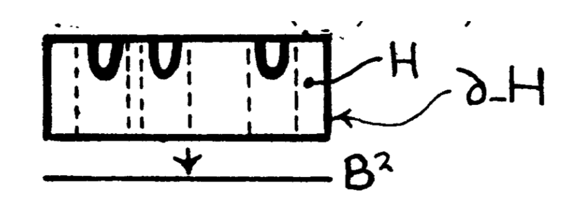
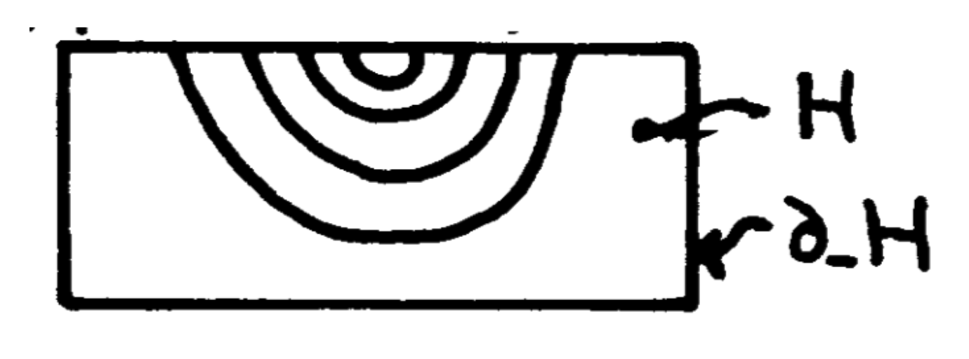
The standard 2-handle is \( (B^2\times D^2,\partial B^2\times D^2) \); its attaching region \( \partial_- \) is \( \partial B^2\times D^2 \); its skin \( \partial_+ \) is \( B^2\times \partial D^2 \), its core is \( B^2\times 0 \). A 2-handle is a pair \[ (H^4,\partial_-H) \ \text{ diffeomorphic to }\ (B^2\times D^2,\partial B^2\times D^2) .\]
An open 2-handle is a manifold diffeomorphic to \( B^2\times \mathring{D^2} \). For a 2-handle (possibly open), the attaching region, the skin and the core are defined by a diffeomorphism with the standard 2-handle (perhaps the open one). In this paper, we can allow ourselves to omit the prefix “2-”; handles of index \( \neq 2 \) appear rarely. Also, we write \( \mathring{D^2} \) where we ought strictly to write \( \operatorname{Int}D^2 \).
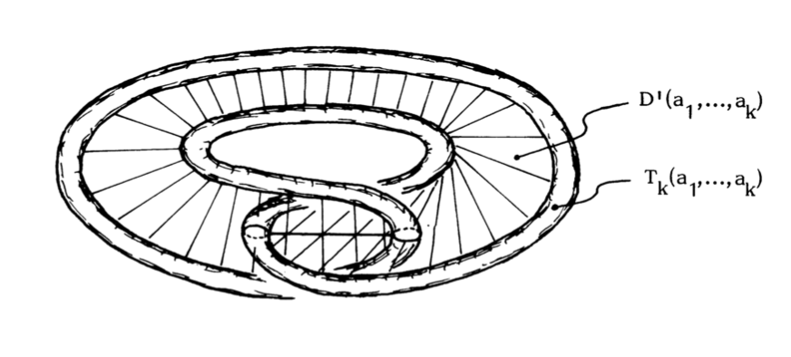
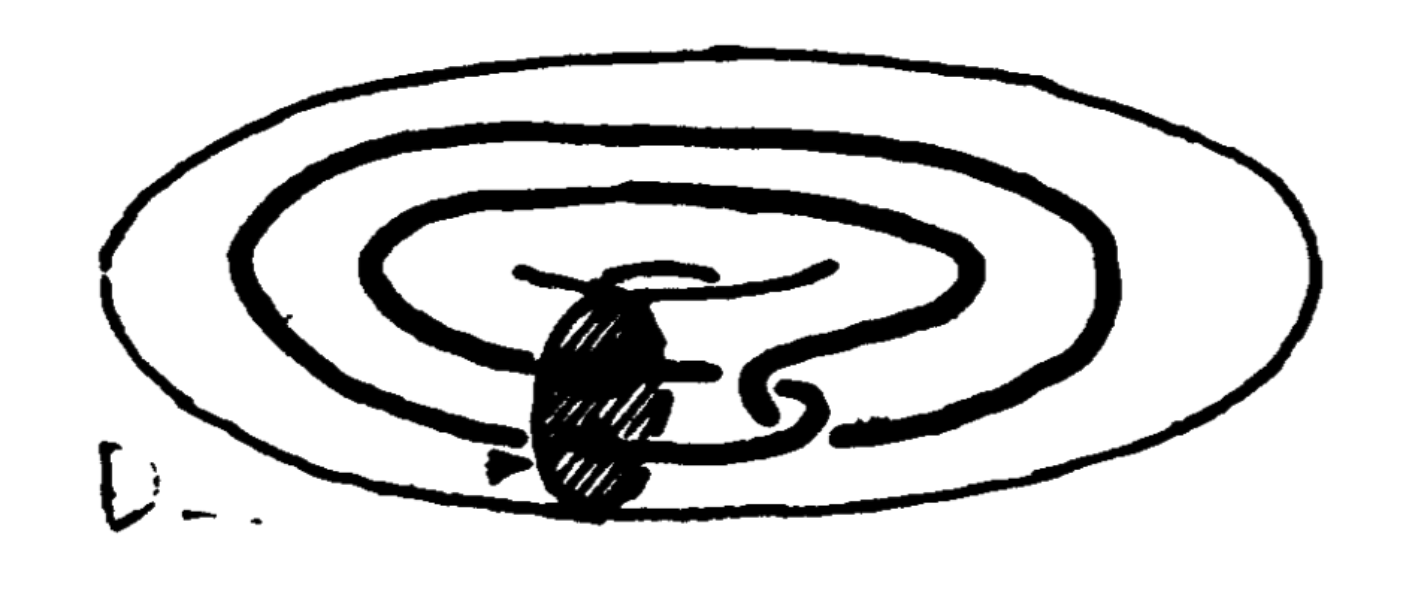
A defect \( X \) in a handle \( (H^4, \partial_-H) \) is a compact submanifold \( X \) of \( H^4\smallsetminus \partial_-H \) such that:
- \( (X, X\cap \partial_+H) \) is a handle where \( \partial_+H \) is the skin of the handle \( (H,\partial_-H) \);
- \( (\partial_+H,X\cap \partial_+H) \) is (degree \( \pm 1 \)) diffeomorphic
to the Whitehead double
\[ (B^2\times S^1,i(B^2\times S^1)) \]
illustrated in Figure 1;
- in the 4-ball \( H^4 \) (with rounded corners), the core \( A^2 \) of the handle \( (X, X\cap \partial_+H) \) is an unknotted disc, that is, \( (H,A) \) is diffeomorphic to \( (B^4, B^2) \).
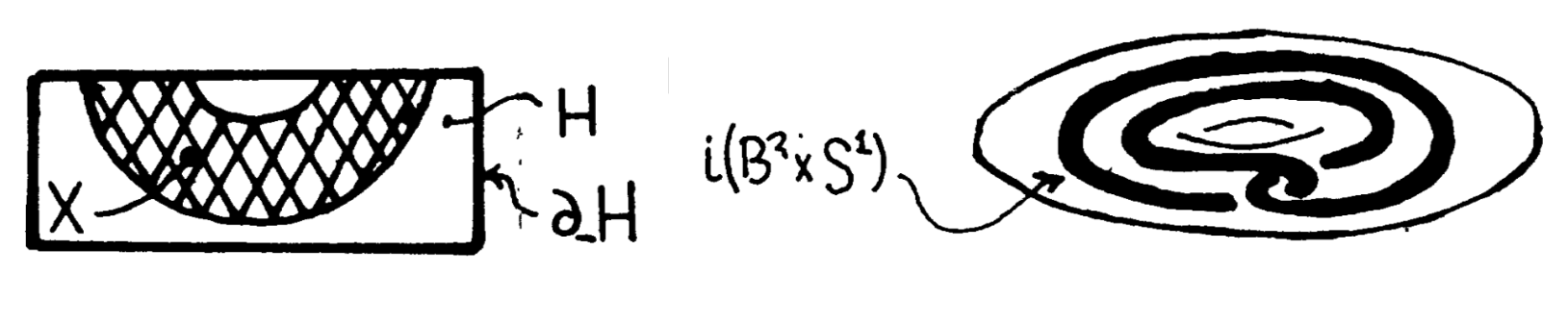
Figure 1.
A multidefect \( X \) in a handle \( (H^4, \partial_-H) \) is a finite sum and union of defects such that for an identification \( (H^4,\partial_-H) \) with \[ (B^2\times D^2, \partial B^2\times D^2) ,\]
project to \( B^2 \) the same number of disjoint discs in \( \operatorname{Int} B^2 \). A multi-defect \( X \) in a handle \( (H^4,\partial H) \) is a finite, disjoint union \( \bigsqcup_i X(i) = X \) of \( \geq 1 \) defects \( X(i) \), that, for a suitable identification \[ (H^4,\partial H) \cong (B^2,\partial B^2) \times D^2 ,\]
are sent, under the projection \( B^2 \times D^2 \to B^2 \), to a disjoint union of discs in \( B^2 \). A multihandle \( (H^4,\partial_-H^4) \) is a disjoint, finite sum of handles. A multiple defect \( X\subset H^4 \) in a multiple handle is a compact subset that gives rise, by intersection, to a multidefect in each handle. With this data, we have the following.
is a diffeomorphism, there exists a diffeomorphism \( \Theta : H\to H^{\prime} \) extending \( \theta \).
Sketch of proof (see [e38]). If we attach a multihandle \( (X^{\prime},\partial_-X^{\prime}) \) to \( H\smallsetminus \mathring{X} \) along the frontier \( \delta X \), in such a way that there exists no extension of \( \theta \) to a diffeomorphism \[ \Theta : H\to (H\smallsetminus \mathring{X})\cup X^{\prime}=H^{\prime} ,\]
we claim that \( (\partial H^{\prime},\partial_-H) \) is diffeomorphic to \( (S^3,\text{solid torus}) \) where the solid torus is tied in a nontrivial knot — in fact, a connected sum of \( k \) nontrivial twist knots, \( 1\leq k\leq |\pi_0(X)| \). ◻
A residual defect \( \Omega \) in a handle \( (H^4,\partial_-H^4) \) is the intersection of a sequence \[X_1\supset \mathring{X_1}\supset X_2\supset \mathring{X_2}\supset X_3\supset \cdots\]
of compact submanifolds of \( H^4\smallsetminus \partial_-H^4 \) such that, for all \( k \), \( (X_k,\delta X_k) \) is a multihandle in which \( X_{k+1} \) is a multidefect. The sequence \( X_1\supset X_2\supset \cdots \) is called a Russian doll of defects.
A Casson handle is a pair \[ (H_\infty^4,\partial_-H_\infty^4) \]
such that there exists a handle \( (H,\partial_-H) \) with a residual defect \( \Omega\subset H \) and an open smooth embedding \[ i_\infty : H_\infty \to H \]
with image \( H\smallsetminus \Omega \), which induces a diffeomorphism \[ i_\infty| : \partial_-H_\infty\to \partial_-H .\]
In other words, \( (H_\infty, \partial_-H_\infty) \) is diffeomorphic to \( (H\smallsetminus \Omega,\partial_-H) \).
The data of \( (H,\partial_-H) \), the Russian doll of defects \( X_i \) and \( i_\infty : H_\infty \to H \), constitute what we will call a presentation of a Casson handle \( (H_\infty,\partial_-H_\infty) \). We will also denote \[ H_k=i_\infty^{-1}(H\smallsetminus \mathring{X_k}) \quad\text{and}\quad \partial_- H_k=\partial_-H_\infty .\]
Then, \( H_\infty=\bigcup_k H_k \). The manifold \( H_k \) is called a tower of height \( k \), its stages are \[ E_j=i_\infty^{-1}(X_{j-1}\smallsetminus X_j) \]
for \( j\leq k \). The restriction of \( i_\infty \) to \( H_k \) will be denoted \( i_k : H_k\to H \).
The skin of \( (H_\infty, \partial_-H_\infty) \) is \[ \partial_+H_\infty=i_\infty^{-1}(\partial_+H) ;\]
moreover, by taking
intersection with \( \partial_+H_\infty \), we define the skin \( \partial_+H_k \)
of \( H_k \) and \( \partial_+E_k \) of \( E_k \). Similarly \( \partial_+X_k=X_k\cap
\partial_+H . \)
A Casson handle \( (H_\infty,\partial_-H_\infty) \) is never compact; we will often encounter the endpoint compactification \( \widehat{H}_\infty \) of \( H_\infty \). Recall that the endpoint compactification \( \widehat{M} \) of a connected, locally connected and locally compact space \( M \) is the Freudenthal compactification that adds to \( M \) the compact 0-dimensional space \( \operatorname{Ends}(M) \) which is the (projective) limit of an inverse system \[ \{\pi_0(M\smallsetminus K)\mid K\subset M \text{ such that } K \text{ is compact}\}. \]
By \( i_\infty \), \( \widehat{H}_\infty \) is identified with the quotient of \( H^4 \) obtained by crushing each connected component of \( \Omega \) to a point. (To verify this, note that \( \pi_0(\Omega) \) with the compact topology is the (projective) limit of an inverse system \( \{\pi_0(U)\mid U \) is an open subset of \( H \) containing \( \Omega\} \).)
We remark that \( \widehat{H}_\infty \) is the Alexandroff compactification by a point, exactly when \( \Omega\subset H \) is connected, or if each successive multiple defect \( X_i \) is a single defect. The reader who feels discombobulated by all the complexities to come may be interested in restricting themselves at first to this case, which already contains all the geometric ideas.
\( \widehat{H}_\infty \) has all the local homological properties of a manifold; it is what we call a homology manifold. But its formal boundary, the closure of \( \partial H_\infty \), is not a topological manifold near its ends. For example, if \( \Omega \) is connected, by definition, \( \partial H_\infty \) (which is homeomorphic to \( \partial H\smallsetminus \partial_+\Omega \)) is one of the contractible 3-manifolds of J. H. C. Whitehead [e1], [e2], with a nontrivial \( \pi_1 \)-system at infinity. \[ \partial_+\Omega\subset \partial H\cong S^3 \]
is a Whitehead compactum. In the general case, \( \partial_+\Omega \) is called a ramified Whitehead compactum. Thus, \( (\widehat{H\smallsetminus \Omega},\partial_-H) \) has no chance of being a topological handle. On the other hand, \[ H\smallsetminus (\partial_+H\cup \Omega) \]
is homeomorphic to \( B^2\times \mathbb{R}^2 \); this will be the central result of this paper.
The proof of Theorem 2.2 starts with a result of 1979, when Freedman was able to construct a smooth 4-manifold \( M \) without boundary which is not homeomorphic to \( S^3\times \mathbb{R} \) that is however the image of a proper map of degree \( \pm 1 \), \( S^3\times \mathbb{R}\to M \) (see [1] and [e34]).
A Casson tower of height \( k \), or more briefly \( C_k \), is a pair diffeomorphic to \( (H\smallsetminus \mathring{X_k},\partial_-H) \) where \( X_1\supset X_2\supset \cdots \) is a Russian doll of defects in a handle \( (H,\partial_-H) \).
- \( \partial_-H_{12}^{\prime}=\partial_-H_6 \).
- \( H_{12}^{\prime}\smallsetminus \partial_-H_6\subset \operatorname{Int}H_6 \).
- \( H_{12}^{\prime}\smallsetminus H_6^{\prime} \) is contained in a disjoint union of balls in \( \operatorname{Int}H_6 \), one ball for each connected component.
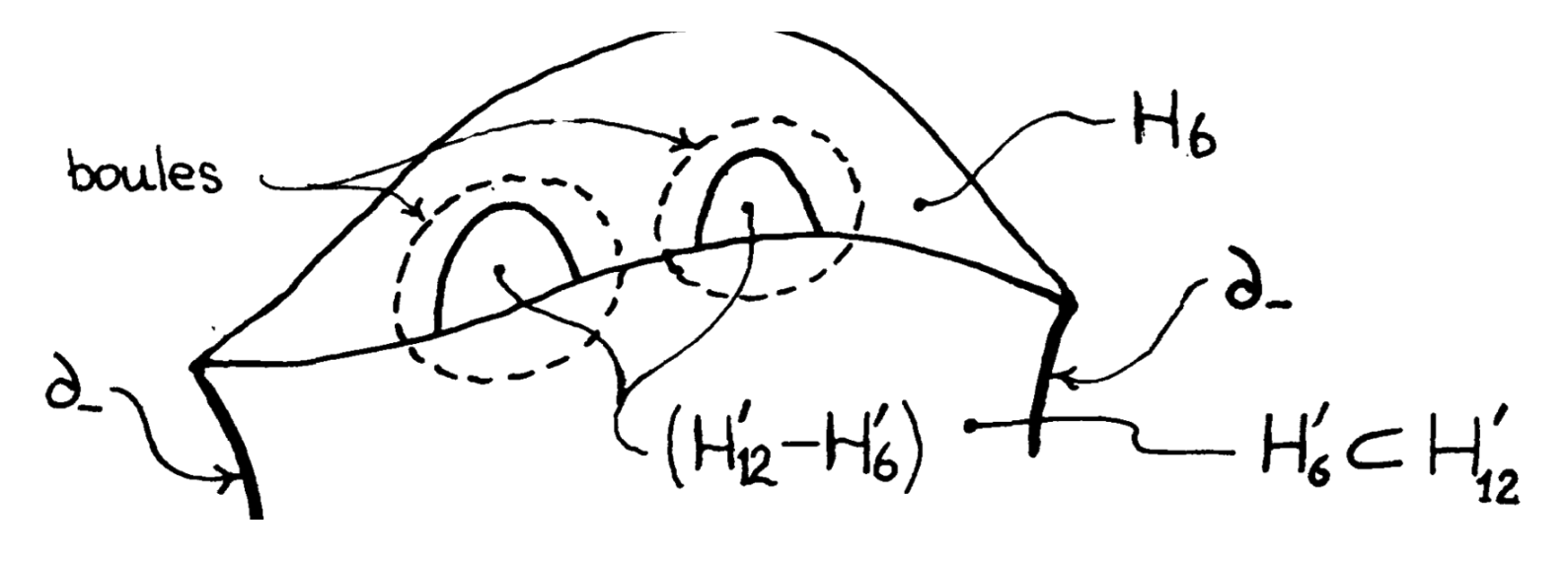
Figure 5.
Condition (3) is related to the fact that, for each Casson tower \[ (H_k,\partial_-H_k) ,\]
the manifold \( H_k \) can be expressed as a regular neighbourhood of a 1-complex, compare [e38]. Figure 5 shows a schematic diagram of Freedman which summarises Theorem 2.3.
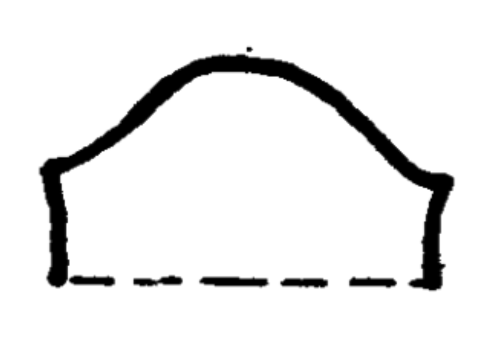
In Section 3, Figure 6 will represent a \( C_6 \), and Figure 7 will represent a \( C_{12} \), etc. From the point of view of the representation of corners on the boundary, it might be better to use Figure 8.
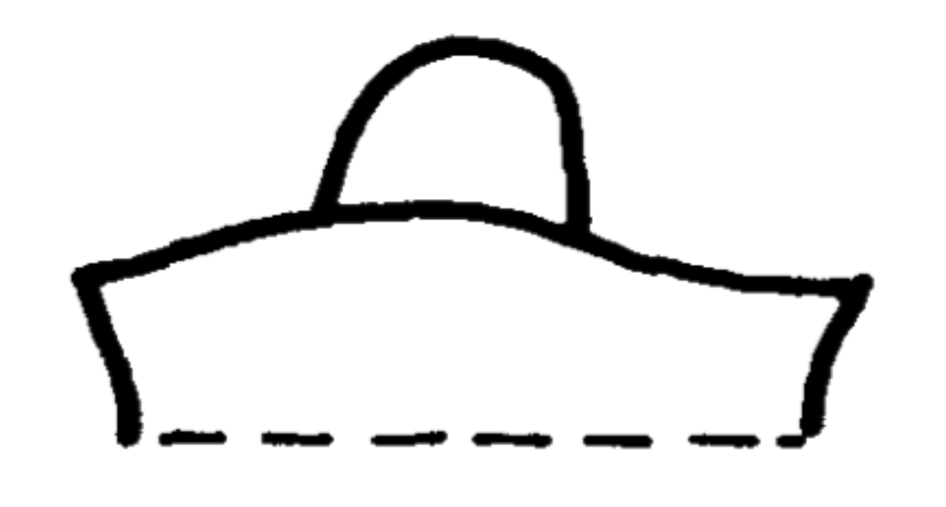
Figure 7.
The method of Freedman [1] (compare [e34]) allows one to give a proof of Theorem 2.3. However, it is slightly more detailed than the analogues in [1], [e34]. We will not cover this point in this paper (see [e37] for an excellent write up of the mitosis theorem (finite version, Theorem 2.3).

Figure 8.
Since we are going to use Theorem 2.3 often, it is convenient to make the following:
- \( H_{k-1}^{\prime}=H_{k-1} \) if \( k\geq 1 \).
- \( \overline{H^{\prime}_\infty}\smallsetminus H_{k-1}^{\prime}\subset (\operatorname{Int} H_k)\smallsetminus H_{k-1} \).
- The closure \( \overline{H_\infty^{\prime}} \) of \( H_\infty^{\prime} \) in \( H_\infty \) is the endpoint compactification of \( H_\infty^{\prime} \).
This infinite version, Theorem 2.5, follows from the finite version, Theorem 2.3, by an infinite repetition. One sufficiently shrinks balls given by Theorem 2.3 to ensure the condition (3) of Theorem 2.5.
3. Architecture of topological coordinates
The open Casson handle \( M \) will be identified with \( N\smallsetminus \partial_+N \) where \( (N,\partial_-N) \) is a Casson handle (not open). Let \( \widehat{N} \) be the endpoint compactification \( \text{of } N \). Subtracting from \( N \) the (topological) interior of a collar neighbourhood of \( \partial_+N \) in \( N \), very pinched towards the ends \( \text{of } N , \) we obtain a Casson handle \[ (H_\infty, \partial_-H_\infty)\subset (M,\partial M)\subset (N,\partial_-N) \]
whose closure in \( \widehat{N} \) is the endpoint compactification \( \widehat{H}_\infty \) of \( H_\infty \). We fix a presentation of \( (H_\infty, \partial_-H_\infty) \).
We will construct a ramified system of Casson handles in \( (N,\partial_-N) \), that, in some way, explores its interior.
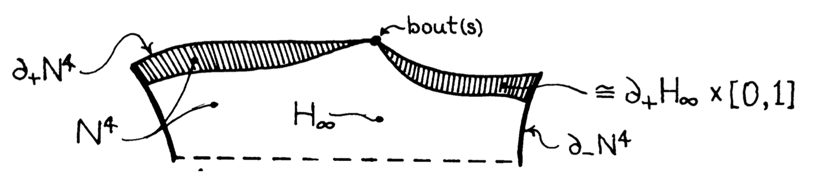
Figure 9.
3.1. Construction
contained in \( (H_\infty,\partial_-H_\infty) \), whose presentation consists of an embedding \[ i_\infty(a_1,\ldots,a_k) : H_\infty(a_1,\ldots,a_k)\to B^2\times D^2, \]
and a Russian doll of defects \( X_i(a_1,\ldots,a_k) \), in the standard handle \( B^2\times D^2 \) such that (for (1)–(5), see the right figure of Figure 10):
- \( H_\infty=H_\infty(\emptyset) \) (case \( k=0 \)) as a presented Casson handle.
- \( H_\infty(a_1,\ldots,a_k,1)=H_\infty(a_1,\ldots,a_k) \).
- \( H_k(a_1,\ldots,a_k,0)=H_k(a_1,\ldots,a_k) \) (recall that \( H_k \) are sets of 6-stages).
- The closure
\[ \overline{H}_\infty(a_1,\ldots,a_k,0)
\quad\text{in}\quad
\widehat{H}_\infty \]
is an endpoint compactification of \( H_\infty(a_1,\ldots,a_k,0) \).
- \( \overline{H}_\infty(a_1,\ldots,a_k,0)\smallsetminus H_k(a_1,\ldots,a_k)\subset \mathring{H}_{k+1}(a_1,\ldots,a_k)\smallsetminus H_k(a_1,\ldots,a_k) \).
- \( i_k(a_1,\ldots,a_k,0)=i_k(a_1,\ldots,a_k) \), so \( X_k(a_1,\ldots,a_k,0)=X_k(a_1,\ldots,a_k) \).
- The intersection of \( X_{k+1}(a_1,\ldots,a_k,0) \) and \( X_{k+1}(a_1,\ldots,a_k) \) is empty, and their union is a multiple defect in \( X_k(a_1,\ldots,a_k) \).
- (Without Change of Notation 2.4) We also require a coherence condition on the total Russian doll assumed by (7), that is to say \( \{X_k\} \), where \( X_k=\bigcup X_k(a_1,\ldots,a_k) \). To formulate it, we momentarily suspend the reindexing convention (Change of Notation 2.4) and write \( T_k=\partial_+X_k \). The condition is that there exists an interval \( J\subset \partial D^2 \) such that, for all \( t\in J \), the meridional disc \( B_t=B^2\times t \) of the solid torus \( B^2\times \partial D \) meets the multiple solid tori \( T_k \) ideally, in the sense that each connected component of \( B_t\cap T_k \) is a meridional disc of \( T_k \), that meets \( T_{k+1} \) in an ideal fashion illustrated in the left figure of Figure 10.
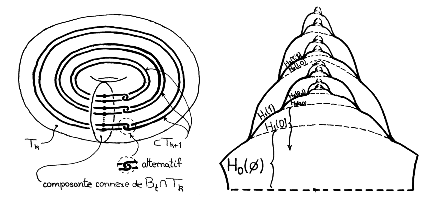
Figure 10.
Execution of Construction 3.1 (by induction on \( k \)). We start with \( H_\infty(\emptyset)=H_\infty \). Having defined a presented handle for every sequence of length \( \leq k \), we define them for every sequence \( (a_1,\ldots,a_k,1) \) by (2). Next, we define \( H_\infty(a_1,\ldots,a_k,0) \) by the mitosis theorem (infinite version, Theorem 2.5). This assures that conditions (3), (4) and (5) are met. It remains to define the presentation of the Casson handle \( (H_\infty(a_1,\ldots,a_n,0),\partial_-H_\infty) \) in such a fashion that the two last conditions (6) and (7) are satisfied. To define \( i_\infty(a_1,\ldots,a_k,0) \), it is convenient to graft, onto \( i_k(a_1,\ldots,a_k) \), a presentation the near part of the Casson handle \[ (H_\infty(a_1,\ldots,a_k,0), \, \partial_-H_\infty) ,\]
to know the Casson multihandle \[ \bigl(H_\infty(a_1,\ldots,a_k,0)\smallsetminus\mathring{H}_k(a_1,\ldots,a_k,0),\delta H_k(a_1,\ldots,a_k,0)\bigr), \]
where exceptionally \( \ \mathring{}\ \) and \( \delta \) denote the interior and the frontier in \( H_\infty(a_1,\ldots,a_k,0) \) rather than in \( \widehat{N} \). The grafting is done with the help of Lemma 2.1. The last condition (7) is assured afterwards by an isotopy in \( \mathring{X}_k(a_1,\ldots,a_k) \). Having (1) to (7), the reader will know how to arrange that (8) is also satisfied. ◻
gives a Casson handle with an obvious presentation. Moreover, the closure \[ \overline{H}_\infty(a_1,a_2,\dots) \]
is the endpoint compactification (exercise). Thus, we have a vast collection of Casson handles in \( N \), conveniently nested.
Of the system of handles \[ (H_\infty(a_1,\ldots,a_k), \partial_-H_\infty) ,\]
we especially use their skins \( \partial_+H_\infty(a_1,\ldots,a_k) \). The union \[ P^3=\bigcup\partial_+H_\infty(a_1,\ldots,a_k) \]
of the skins is what one calls a branched manifold in \( N^4 \), since near every point \( P^3\smallsetminus \partial_-H_\infty \), the pair \( (N^4,P^3) \) is \( C^1 \)-isomorphic (same as \( C^\infty \)-isomorphic, after some work that we leave to the reader) to the product of \( \mathbb{R}^2 \) with the model of branching \( (\mathbb{R}^2,Y^1) \) where \( Y^1 \) is the union of two smooth curves (isomorphic to \( \mathbb{R}^1 \)), properly embedded in \( \mathbb{R}^2 \) and which have in common exactly one closed half-line. One observes without difficulty that the closure \( \overline{P} \) of \( P \) in \( \widehat{N} \) is the endpoint compactification of \( P \).
The branched manifold \( P \) splits along the singular points into compact manifolds: \begin{align*} P_k(a_1,\ldots,a_k) &=\partial_+E_k(a_1,\ldots,a_k)\\ &=E_k(a_1,\ldots,a_k)\cap \partial_+H_\infty(a_1,\ldots,a_k). \end{align*}
Thus, \( P_k(a_1,\ldots,a_k) \) is the skin of the \( k \)-th stage of \( (H_\infty(a_1,\ldots,a_k),\partial_-H_\infty) \).
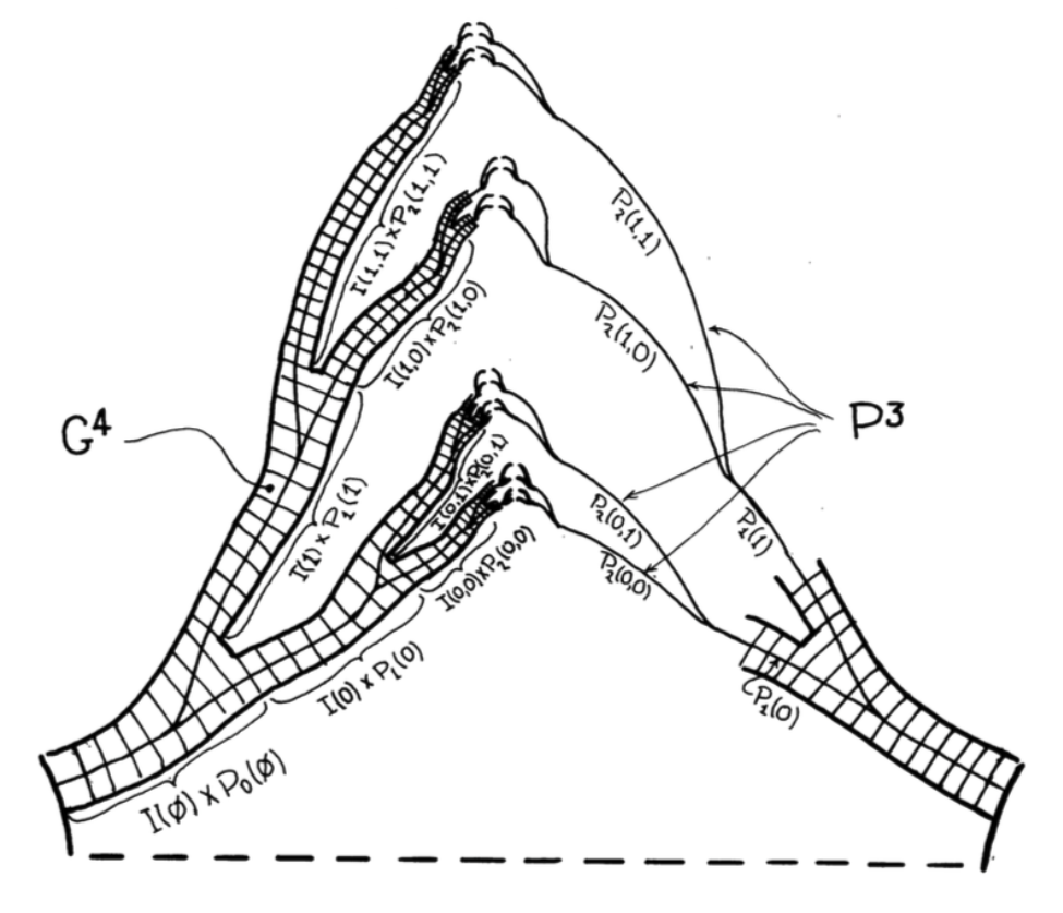
3.2. Construction of the design \( G^4 \) (see Figure 11)
For \( P^3 \), we construct a neighbourhood \( G^4 \) in \( N^4 \) called the design, which has a decomposition \( \mathcal{I} \) of \( G^4 \) into disjoint intervals, satisfying the following.
- For every interval \( I_\alpha \) of \( \mathcal{I} \), the intersection
\[ I_\alpha\cap \partial_-N \]
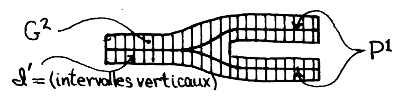
is \( I_\alpha \) or the empty set. A neighbourhood of \( I_\alpha \) in \( (G^4,P^3;\mathcal{I}) \) is isomorphic to the product of \( \mathbb{R}^2 \) with an open 2-dimensional model \( (G^2,P^1;\mathcal{I}^{\prime}) \) as in Figure 12.
- The closure \( \overline{G} \) of \( G \) in \( \widehat{N} \) is its endpoint compactification, and hence coincides with \( G\cup \overline{P} \).
It follows by combining, quite naively, two bicollars of genuine submanifolds of \( P^3 \). On the other hand, we clearly are permitted to suppose that \( G^4 \) contains the collar \( N\smallsetminus \mathring{H}_\infty \) of \( \partial_+N \).
The design \( (G^4,\mathcal{I}) \) decomposed into intervals splits in a canonical fashion (along the 3-manifold formed by the exceptional intervals of \( \mathcal{I} \) having interior points on \( \partial G^4 \)) into genuine trivial \( I \)-bundles \[ I(a_1,\ldots,a_k)\times P_k(a_1,\ldots,a_k) ,\]
where \( I(a_1,\ldots,a_k) \) is a 1-simplex and \[ (\text{its centre})\times P_k(a_1,\ldots,a_k)\subset G^4 \]
is nearly the natural inclusion \( P_k(a_1,\ldots,a_k)\subset G^4 \). More precisely, the two embeddings are isotopic in \( G^4 \) by an isotopy which moves only a collar of the boundary of \( P_k(a_1,\ldots,a_k) \). It is convenient to give a normal orientation to \( P^3 \) in \( N^4 \) (towards the exterior), to deduce from it the orientation of the 1-simplices \( I(a_1,\ldots,a_k) \).
3.3. Construction of \( g : G^4\to B^2\times D^2 \)
This \( g \) will be a smooth embedding which will reveal the structure of \( G^4 \). We choose, by recurrence, linear embeddings \( I(a_1,\ldots,a_k)\subset (0,1] \) conserving the orientation. To start, \( I(\emptyset)\subset (0,1] \) ends at 1. Suppose now these embeddings have been defined for all sequences of length \( \leq k \). Then, we embed \( I(a_1,\ldots,a_k,0) \) and \( I(a_1,\ldots,a_k,1) \) respectively on the initial third and the final third of the interval \( I(a_1,\ldots,a_k)\subset (0,1] \).
The central third of \( I(a_1,\ldots,a_k) \) is a closed interval that we may call \( J(a_1,\ldots,a_k) \). The complement in \( I(\emptyset) \) of all the open intervals \( \mathring{J}(a_1,\ldots,a_k) \) is then a compact Cantor set in \( (0,1] \).
On the other hand, we claim that the embeddings \[ i_k(a_1,\ldots,a_k)| : \partial_+H_k(a_1,\ldots,a_k)\to B^2\times \partial D^2 \]
define together a smooth map \( i : P\to B^2\times \partial D^2 \). Let \[ \varphi : (0,1]\times B^2\times \partial D^2\to B^2\times D^2 \]
be the embedding \( (t,x,y)\mapsto (x,ty) \). We will have the tendency to identify domain and codomain by \( \varphi \).
We define \( g : G^4\to B^2\times D^2 \) on \[ I(a_1,\ldots,a_k)\times P_k(a_1,\ldots,a_k) \]
by the rule that \( (t,x)\mapsto \varphi(t,i(x)) \). For that definition to make sense, we have to first adjust, by isotopy, the trivialisation given by the \( I \)-fibres \[ I(a_1,\ldots,a_k)\times P_k(a_1,\ldots,a_k) \]
in \( (G^4,\mathcal{I}) \), a routine task that is left to the reader.
3.4. Construction of \( g_0 : G_0^4\to B^2\times D^2 \)
By uniqueness of collars, we can arrange \( g \) and \( g_0 \) so that \( g_0 \) sends \( C^4\smallsetminus \mathring{G}^4 \) to \[ (B^2\smallsetminus \lambda B^2)\times \mu D^2 ,\]
where \( \lambda\in (0,1] \) is near to 1 and \( \mu \) to the initial point of \( I(\emptyset) \). This completes the construction of \( g_0 : G_0^4\to B^2\times D^2 \). Looking near \( g_0 \) and its image, we will claim that we have completely described the closure \( \overline{G_0^4} \) of \( G_0^4 \) in \( \widehat{N}^4 \).
3.5. The image \( g_0(G_0^4)\subset B^2\times D^2 \)
- \( T(a_1,\ldots,a_k)\equiv T_k(a_1,\ldots,a_k)=\partial_+X(a_1,\ldots,a_k) \), a multisolid torus \( \subset B^2\times \partial D^2 \).
- \( T_*(a_1,\ldots,a_k)=\varphi(J(a_1,\ldots,a_k)\times T(a_1,\ldots,a_k))\subset B^2\times \mathring{D}^2 \), a radially thickened copy of \( T(a_1,\ldots,a_k) \), called a hole.
- \( B_*=\lambda B^2\times \mu D^2 \) (see definition of \( g_0 \)), called the central hole.
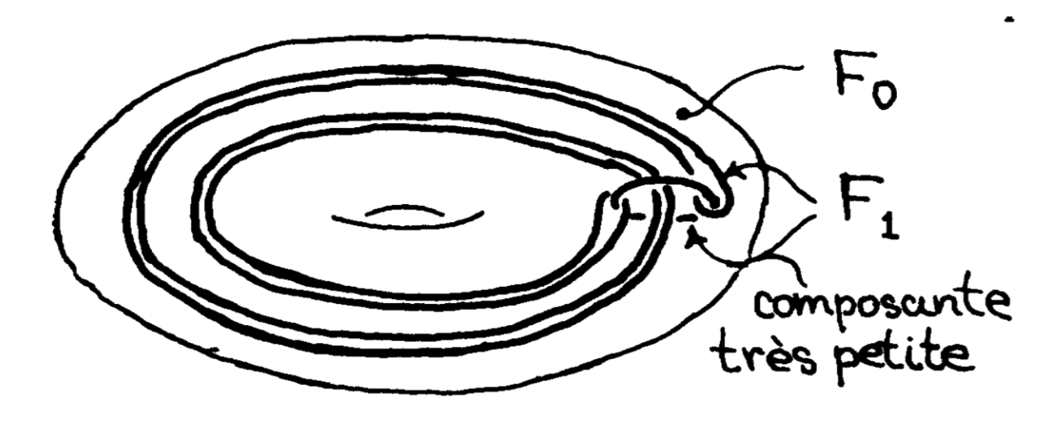
- \( F_k=\bigcup\{\varphi(I(a_1,\ldots,a_{k-1})\times T(a_1,\ldots,a_k))\mid k \text{ fixed}\} \); the frontiers \( \delta F_k \), \( k\geq 2 \), are indicated in dashed lines in the right-hand figure below.
- \( (B^2\times D^2)_0=(B^2\times D^2\smallsetminus \mathring{B}_*)\smallsetminus \bigcup\{\mathring{T}_*(a_1,\ldots,a_k)\} \), called the holed standard handle.
- \( W_0=\bigcap_k F_k \), a compactum in \( (B^2\times D^2)_0 \).
With this notation, we claim that the image \( g_0(G_0^4) \) is \( (B^2\times D^2)_0\smallsetminus W_0 \).
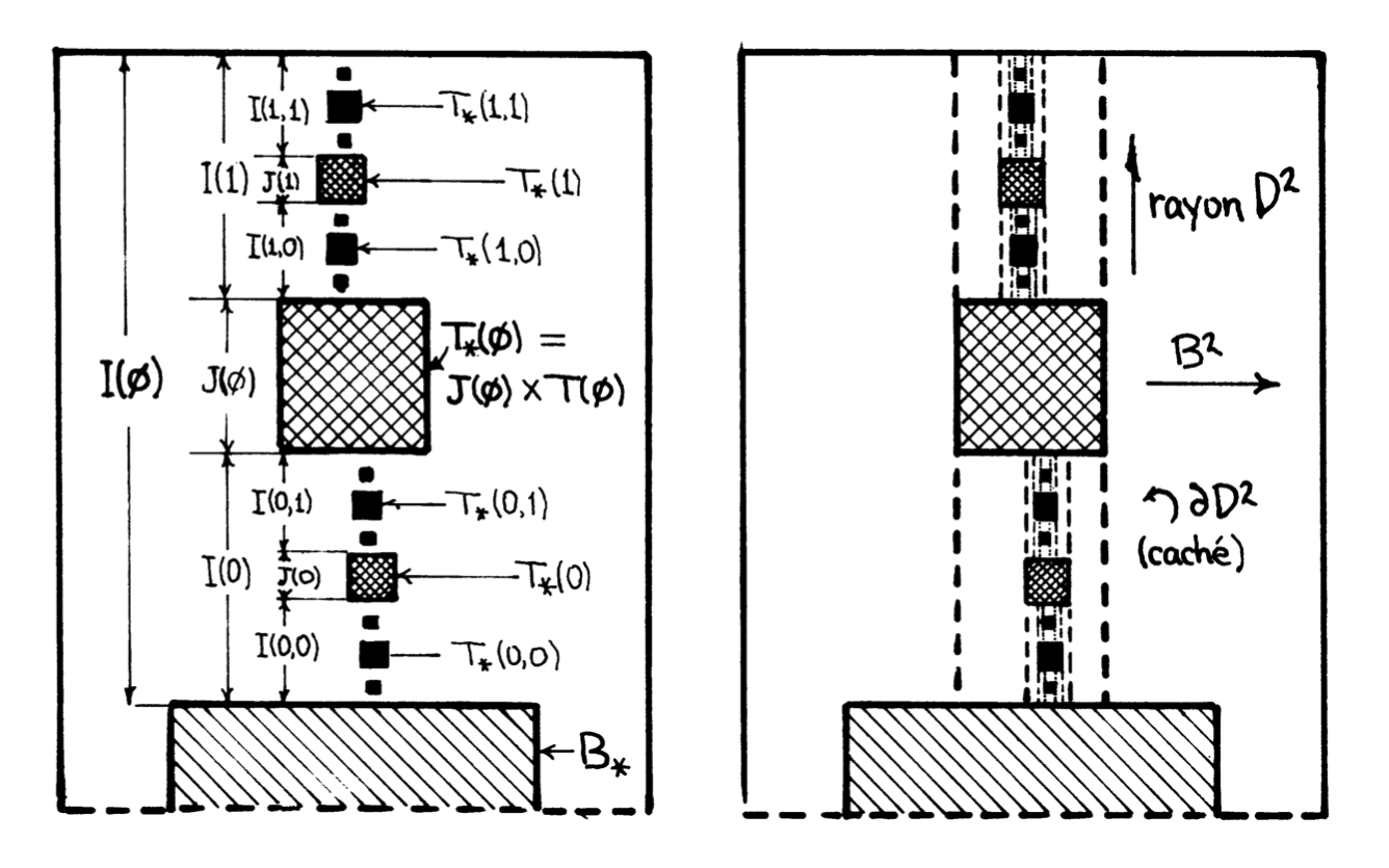
Figure 13.
3.6. The main diagram
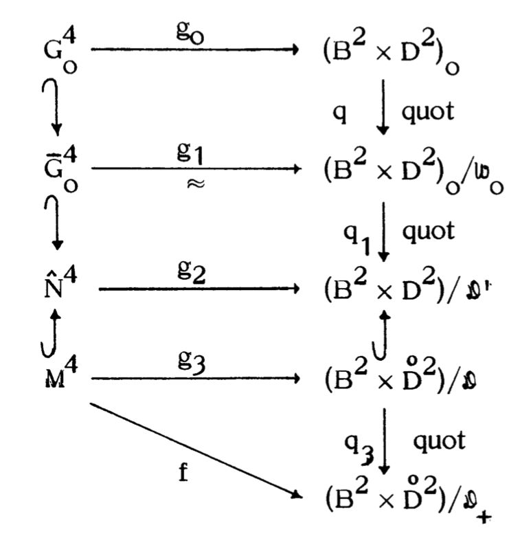
is homeomorphic to \( B^2\times \mathring{D}^2 \) (by the methods of Bing) will appear in Section 4. The proof that \( f \) is approximable by homeomorphisms is postponed to Section 5.
3.7. Construction of \( \mathcal{W}_0 \) and \( g_1 \)
induces a homeomorphism \[ ((B^2\times D^2)_0\smallsetminus W_0)^\wedge\to (B^2\times D^2)_0/\mathcal{W}_0. \]
We already know that \( \widehat{G}_0 \) is identified with \( \overline{G}_0\subset \widehat{N} \). We define the homeomorphism \( g_1 \) as a composition of homeomorphisms: \[ g_1 : \overline{G}_0\to \widehat{G}_0\xrightarrow{\hat{g}_0} ((B^2\times D^2)_0\smallsetminus W_0)^\wedge\to (B^2\times D^2)_0/\mathcal{W}_0. \]
3.8. Construction of \( \mathcal{D}^{\prime} \) and \( g_2 \)
we must extend \[ q_1g_1 : \overline{G}_0\to (B^2\times D^2)/\mathcal{D}^{\prime} \]
to each connected component \( Y \) of \( \widehat{N}\smallsetminus \overline{G}_0 \). Its frontier \( \delta Y \) is identified by \( g_1 \) to the quotient in \[ (B^2\times D^2)_0/\mathcal{W}_0 ,\]
either of \( \partial B_* \), or of a boundary of a connected component of a hole \( T_*(a_1,\ldots,a_k) \). By definition, \( g_2(Y) \) is the image in \( (B^2\times D^2)/\mathcal{D} \) of this boundary. It is easy to check the continuity of \( g_2 \).
Next, \( g_3 \) and \( \mathcal{D} \) in the main diagram are defined by restriction. The design \( G^4 \) has led us inexorably to define \[ g_3 : M^4\to B^2\times \mathring{D}^2/\mathcal{D} ,\]
which compares the open Casson handle \( M^4 \) with a very explicit quotient of the open handle \( B^2\times \mathring{D}^2 \).
The decomposition \( \mathcal{D} \) which specifies this quotient has noncellular elements, that is, the holes \( T_*(a_1,\ldots,a_k) \), each of which has the homotopy type of a circle. Therefore the quotient map \[ B^2\times \mathring{D}^2\to B^2\times \mathring{D}^2/\mathcal{D} \]
is certainly not approximable by homeomorphisms. One can also check that the Čech cohomology \( \check{H}^2 \) of the quotient is of infinite type.
The construction of \( \mathcal{D}_+ \) below repairs this terrible defect; it will be constructed by hand; \( \mathcal{D}_+ \) will be less fine than \( \mathcal{D} \), which will enable us to define \( f=q_3\circ g_3 \) without effort.
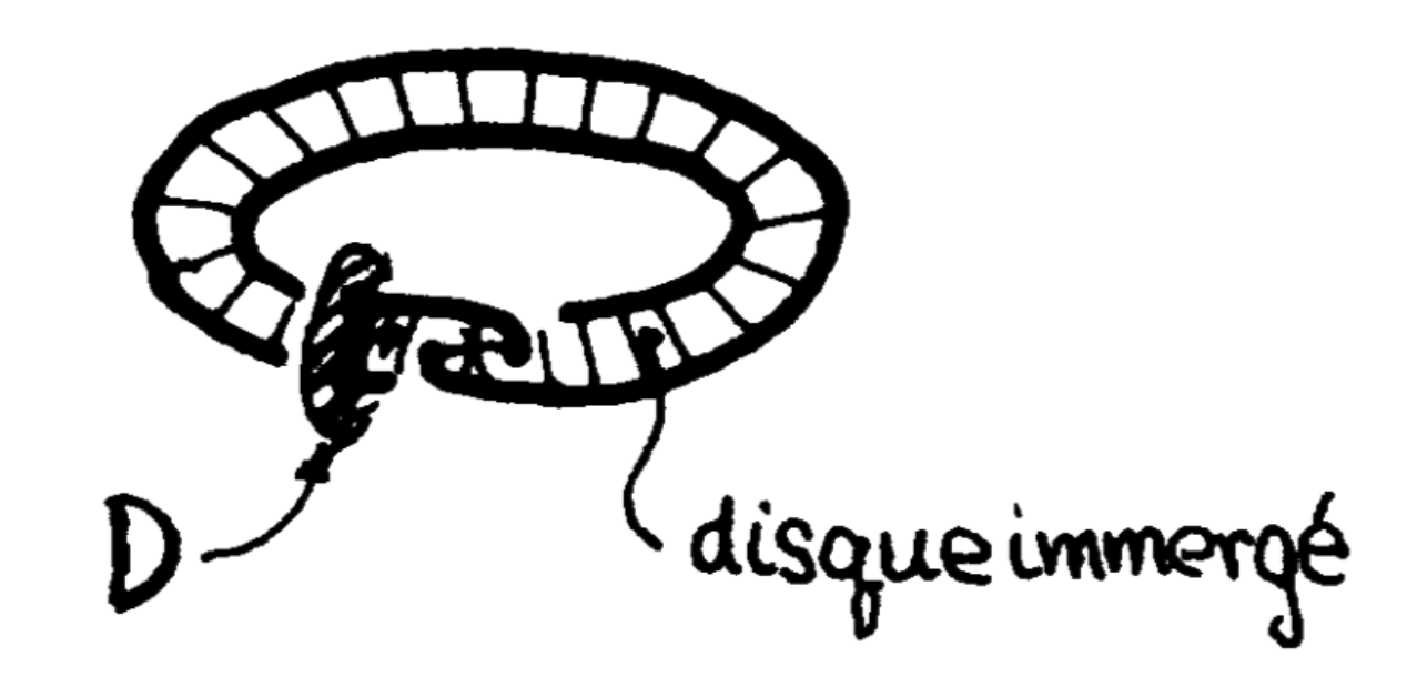
3.9. Construction of \( \mathcal{D}_+ \)
Its connected components define a decomposition \( \mathcal{W} \) of \( B^2\times \mathring{D}^2 \). We have known since the 1950s how to show that \( B^2\times \mathring{D}^2/\mathcal{W} \) is homeomorphic to \( B^2\times \mathring{D}^2 \), see Section 4.
For the requirements of the next paragraph, the quotient \( (B^2\times \mathring{D}^2)/\mathcal{D}_+ \) must be a quotient of \( B^2\times \mathring{D}^2/\mathcal{W} \) by a decomposition whose elements are the connected components of \[ \bigcup \{q(T_*(\alpha))\cup E(\alpha)\mid \alpha\text{ a finite dyadic sequence}\}. \]
Here \( \{E(\alpha)\} \) is a collection of disjoint, topologically flat multi-2-discs such that for each finite dyadic sequence \( \alpha \), the intersection \[ E(\alpha)\cap \biggl(\bigcup_{\alpha^{\prime}}q(T_*(\alpha^{\prime}))\!\biggr) \]
is
- the boundary \( \partial E(\alpha) \); and
- a multilongitude of \( \partial T_*(\alpha) \) far from \( W \) (each
connected component of
\[ q(T_*(\alpha))\cup E(\alpha) \]
is then contractible).
Moreover, we want that the diameter of the connected components of \( E(a_1,\ldots,a_k) \) tends towards 0 (on each compact set) as \( k\to \infty \). Section 4 does not demand any more than this and visibly, \( \{E(\alpha)\} \) specifies \( \mathcal{D}_+ \).
The specification of \( \{E(\alpha)\} \) is unfortunately tedious. \( E(\alpha) \) will be the faithful image \( q(D(\alpha)) \) of a multidisc in \( B^2\times \mathring{D}^2 \). For fundamental group reasons, the multidisc \( D(\alpha) \) is obliged to meet \( W \), but, to assure flatness of \( q(D(\alpha)) \) (proved in Section 4), it must be a well behaved meeting, permitted by (7) and (8) of Construction 3.1.
We have \( T_k=\bigcup_\alpha T_k(\alpha) \); conditions (6) and (7) of Construction 3.1 assure that \( T_k \) is a multisolid torus of which certain connected components constitute \( T_k(\alpha) \). We have \[ \bigcap_k T_k=p(W) ,\]
which is a ramified Whitehead compactum in \( B^2\times \partial D^2 \).
To start, we specify (simultaneously and independently) in \( B^2\times \partial D^2 \), (topologically) immersed, locally flat discs \( D^{\prime}(\alpha) \) which will be the projection \( p(D(\alpha))=D^{\prime}(\alpha) \). We assume easily the two properties (a) and (b), where (b) uses (8) of Construction 3.1.
(a) \( D^{\prime}(a_1,\ldots,a_k) \) is a disjoint union of immersed discs in \( T_{k-1} \), with as their only singularities, an arc of double points for each, above \[ T_k(a_1,\ldots,a_k) .\]
The boundary \[ \partial D^{\prime}(a_1,\ldots,a_k) \]
is formed from one longitude of each connected component of \( \partial T_k(a_1,\ldots,a_k) \). The double points of \( D^{\prime}(a_1,\ldots,a_k) \) are outside \( \mathring{T}_k(a_1,\ldots,a_k) \).
(b) For each \( l\geq k \), the intersection \[ \mathring{D}^{\prime}(a_1,\ldots,a_k)\,\cap\,T_l \]
is a multidisc (embedded in \( T_k(a_1,\ldots,a_k) \)) of which each connected component \( D_0 \) is a meridional disc of \( T_l \) that meets the solid tori of the next generator (\( T_{l+1/6} \) with our revised indexing of Change of Notation 2.4) ideally (see the left-hand figure of Figure 10).
By resolving the double points of \( D^{\prime}(\alpha) \), which we have to embed in \[ (0,1)\times B^2\times \partial D^2\subset B^2\times D^2, \]
specifying the first coordinate by a convenient function \( \rho(\alpha) : D(\alpha)\to (0,1) \).
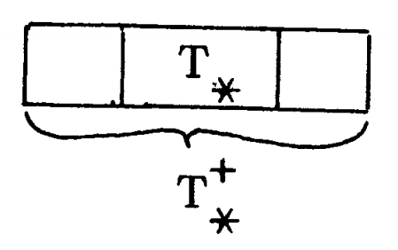
We will embed a single \( D(\alpha) \) at a time (following some chosen order). We embed first \( D(a_1,\ldots,a_k) \) closer and closer (by a secondary induction). Some notation: \begin{equation*} \eqalign{ T_*^+(a_1^{\prime},\ldots,a_l^{\prime})&=J(a_1^{\prime},\ldots,a_l^{\prime})\times T(a_1^{\prime},\ldots,a_{l-1}^{\prime}),\cr F_l^*=p^{-1}(p(F_l))&=(0,1)\times T_l,\cr W^+=p^{-1}(p(W))&=(0,1)\times \biggl(\bigcap_k T_k\biggr). } \end{equation*}
One can easily check that, for \[ D(a_1,\ldots,a_k) ,\]
the properties (c) and (d) for \( l > k \), of which (d) for \( l \) is only provisional.
(c) \( D(a_1,\ldots,a_k) \) is embedded, is contained in \[ I(a_1,\ldots,a_{k-1})\times T(a_1,\ldots,a_{k-1}), \]
and is disjoint from \( B_* \) and from \[ \bigcup\{T_*^+(\alpha^{\prime})\mid \alpha^{\prime}\neq (a_1,\ldots,a_k)\} .\]
The boundary \( \partial D (a_1,\ldots,a_k) \) is in a single level \( t\times B^2\times \partial D^2 \), where \( t\in \mathring{J}(a_1,\ldots,a_k) \).
(d) Each connected component of the multidisc \[ F_l^+\cap D(a_1,\ldots,a_k) \]
is in a single level \( t\times B^2\times \partial D^2 \); this level is disjoint from each box \( T_*(\alpha^{\prime}) \), and does not contain any other connected component of \( F_l^+\cap D(a_1,\ldots,a_k) \).
For \( l=k \) and \( k+1 \), here are the illustrations of the graph of \( \rho \) in a simple case.
We observed that in pushing \[ D(a_1,\ldots,a_k) \]
vertically, as small as we want, and only on \[ \mathring{F}_l^+\cap D(a_1,\ldots,a_k) ,\]
we can pass from (d) for \( l \) to (d) for \( l+1 \), without losing (c). Therefore, without losing (c), we can pass to the next property.
(e) For each integer \( l > k \), the connected components of the multidisc \[ F_l^+\cap D(a_1,\ldots,a_k) \]
project onto as many disjoint intervals of radius in \( (0,1) \).
This condition assures that, for all \( W\in \mathcal{W} \), the intersection \[ W\cap D(a_1,\ldots,a_k) \]
is an intersection of discs (and so cellular). Therefore \( q(D(a_1,\ldots,a_k)) \) is certainly a disc (compare Theorem 4.4). In Section 4, we will prove by hand that it is a flat disc. If, before \( D(a_1,\ldots,a_k) \), we have already defined (for the main induction) a finite collection of discs \[ D(\alpha_1),\ldots, D(\alpha_n) ,\]
we follow the same construction as above, always staying in a neighbourhood of \( T_*^+(a_1,\ldots,a_k) \) (guaranteed by (c)), disjoint from \( D(\alpha_1)\cup \cdots\cup D(\alpha_n) \) and for all elements of \( \mathcal{W} \) that touch \( D(\alpha_1)\cup\cdots\cup D(\alpha_n) \).
Thus the family \( \{D(\alpha)\} \) of disjoint 2-discs is defined by a double induction and satisfies the properties (a), (b), (c) and (e) with \[ p(D(\alpha))=D^{\prime}(\alpha) .\]
Next \( \{D(\alpha)\} \) defines \( \mathcal{D}_+ \) as already indicated. One easily checks all the properties wanted for \[ q(D(\alpha))=E(\alpha) \quad\text{in}\quad (B^2\times \mathring{D}^2)/\mathcal{W} ,\]
except local flatness of \( E(\alpha) \) which is postponed to Section 4.
3.10. End of the proof that \( M \) is homeomorphic to \( B^2\times\mathring{D}^2 \) (modulo Sections 4 and 5)
in the following fashion. We form the commutative diagram

Therefore, \[ S(f_*)=\{y\in S^4\mid f^{-1}_*(y)\neq \text{ a point}\} \]
is visibly a contractible set.
Also \( S(f_*) \) is nowhere dense. [Here is a proof. The restriction \( f_*| \) is the same as \[ q_3\circ q_1\circ g_1| : M\cap \overline{G}_0^4\to (B^2\times \mathring{D}^2)/\mathcal{D}_+, \]
which is already surjective and \( f_*^{-1}(S(f_*)) \) is contained in the nowhere dense set of \( M\cap \overline{G}_0^4 \) given by \( (\partial G_0)\cup( \)ends of \( G_0^4)\cup g_1^{-1}\bigl(\bigcup_\alpha E(\alpha)\bigr) \).]
Therefore, according to Theorem 5.1, the map \( f_* \) is approximable by homeomorphisms. Next, by Proposition 4.2 (localisation principle), the restriction \[ \operatorname{Int} M^4\to S^4\smallsetminus \{\infty\} \]
is also approximable by homeomorphism. Finally, by Proposition 4.3 (globalisation principle), the map \[f : M\to (B^2\times \mathring{D}^2)/\mathcal{D}_+\]
is approximable by homeomorphisms. Thus Theorem 2.2 is proved modulo Sections 4 and 5.
4. Bing shrinking
We consider a proper surjective map \( f : X\to Y \) between metrisable, locally compact spaces \( X \), \( Y \). Let \[ \mathcal{D}=\{f^{-1}(y)\mid y\in Y\} \]
be the decomposition associated with \( f \). When is \( f \) (strongly) approximable by homeomorphisms, in the sense that for all open coverings \( \mathcal{V} \) of \( Y \), the \( \mathcal{V} \)-neighbourhood \[ N(f,V)=\{g : X\to Y\mid \text{for all }x\in X,\text{ there exists }V\in\mathcal{V}\text{ such that }f(x), g(x)\in V\} \]
contains a homeomorphism?
Since \( f \) induces a homeomorphism \( \varphi : X/\mathcal{D}\to Y \), we see easily that \( f \) is approximable by homeomorphisms if and only if one can find maps \( g : X\to X \) such that \[ \mathcal{D}=\{g^{-1}(x)\mid x\in X\} \]
and that \( f\circ g \) approximates \( f \) (in effect, \( \varphi \) translates \( g \) into a homeomorphism \( g^{\prime} : Y\to X \)). This observation makes the following theorem plausible.
We then say that \( \mathcal{D} \) is shrinkable. We can show a proof by hand [e28], or by Baire category [e35], [e11] (the idea is to find a homeomorphism \( h : X\to Y \) that converges towards \( g \) that determines \( \mathcal{D} \)). The proof also gives:
of \( f \) is approximable by homeomorphisms.
Proof (indication). To approximate \( f_V \), we combine (by the principle \( \mathcal{D}_1 \)) a series of approximations of \( f \); compare ([e23], Section 3.5). I believe that this lemma is not in the literature because, for dimension \( \neq 4 \), we have stronger results [e22], [e32]. However, upon reflection, the complicated argument of [e22] works. In each case that interests us, the reader will be able to find an ad hoc proof that is easier. ◻
and \( f=g\times \operatorname{Id}_{[0,1]} \), where \[ g(1,a_2,a_3,\dots)=(a_2,a_3,\dots), \quad g(0,a_2,a_3,\dots)=(0,0,0,\dots). \]
is approximable by homeomorphisms. Then, \( f \) is approximable by proper maps \( g \) such that
- \( g^{-1}(V)=f^{-1}(V) \),
- \( g_V : g^{-1}(V)\to V \) is a homeomorphism, and
- \( g= f \) on \( X\smallsetminus f^{-1}(V) \).
This principle is easy to establish, because if \( \mathcal{V} \) is the covering of \( V \) by open balls centred on \( y\in V \) and of radius \[ \inf\{ d(y,z)\mid z\in Y\smallsetminus V\}, \]
then every map \[ \gamma : f^{-1}(V)\to V \]
that is in \( N(f_V,\mathcal{V}) \), extends by \( f \) to a map \( g : X\to Y \). In the very special case that \( \mathcal{D} \) is \( \pi_0(K) \) for a compact set \( K\subset X \), the Bing shrinking criterion simplifies as follows. (Then, \( \mathcal{D} \) consists of connected components of \( K \) and the image of \( K \) in \( X/\mathcal{D} \) is 0-dimensional and is identified with \( \pi_0(K) \).)
This condition, modulo localisation principle (Proposition 4.2), is clearly necessary.
For all \( \epsilon > 0 \), one can consider \[ \mathcal{D}_\epsilon=\{D\in \mathcal{D}\mid \operatorname{diam}D\geq \epsilon\}. \]
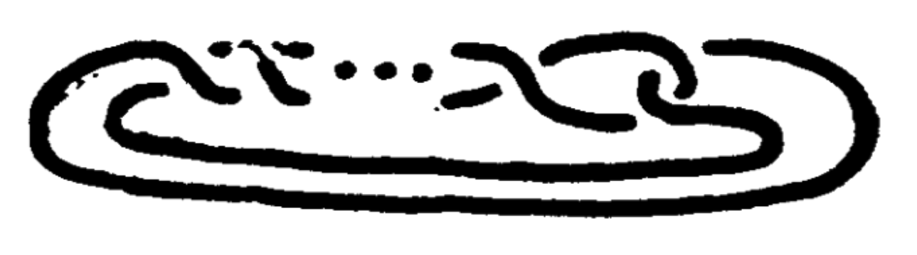
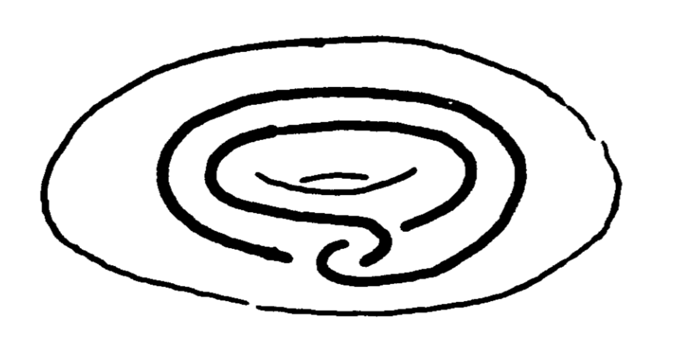
We say that \( \bigcup_{D\in \mathcal{D}_\epsilon} D \) is a closed subset of \( X \). Here is a remarkable but disturbing example where \( \mathcal{D} \) is null, \( \mathcal{D}_\epsilon \) is shrinkable for any \( \epsilon > 0 \), but \( \mathcal{D} \) is not shrinkable. The elements of \( \mathcal{D} \) are the connected components of a compact set \( X=\bigcap_n F_n \) where \( F_0 \) and \( F_1 \) are as illustrated. This image is suitably replicated in each solid torus; \( F_n \) is then \( 2^n \) solid tori. Each \( D\in \mathcal{D} \) is clearly cellular, hence \( \mathcal{D}_\epsilon \) is shrinkable by Lemma 5.2. But, with the help of cyclic covers, one can check that \( \mathcal{D} \) is not shrinkable (see [e12], [e1]).
There are thankfully properties of individual elements, a little stronger than cellularity, which discards this sort of example. For a compact \( A\subset X \), we consider the property \( \mathcal{R}(X,A) \): for each \( \epsilon > 0 \), for every null decomposition \( \mathcal{D} \) of \( X \) containing \( A \), and for all neighbourhoods \( U \) of \( A \), there is a map \( f : X\to X \) with support in \( U \) that shrinks at least \( A \), (that is, \( f(A) \) is a point and \( f|_U : U\to U \) is approximable by homeomorphisms), such that, for all \( D\in \mathcal{D} \), \[ \operatorname{diam} f(D)\leq \max (\operatorname{diam} D,\epsilon). \]
If \( \mathcal{D} \) is fixed in advance, we call the (weaker) property \( \mathcal{R}(X,A;\mathcal{D}) \).
Proof. The proof is an edifying exercise. ◻
Proof of Proposition 4.6. This is \( \mathcal{R}(\mathbb{R}^n,B^k) \) for \( k\leq n \). The proof of \( \mathcal{R}(\mathbb{R}^2,B^1) \) which is indicated by Figure 16.
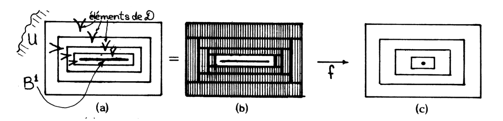
Figure 16.
In (a), every element of \( \mathcal{D} \) that meets the big rectangle has already diameter \( < \epsilon/4 \); if \( D\in \mathcal{D} \) meets a gap between successive rectangles, it is disjoint from the rectangle after. We set \( f(B^1)=0 \), and \( f=\operatorname{Id} \) outside the biggest rectangle (which is in \( U \)); \( f \) is linear on each vertical interval in a rectangle of (b) and also linear on each 1-cell of the rectangular cellulation in (b) of (big rectangle\( \smallsetminus B^1 \)). Moreover, \( p\circ f=p \) where \( p \) is the projection to the \( y \)-axis (the \( \mathbb{R}^{n-k} \) normal to \( B^k \)). Finally, the size of the image of each of the vertical rectangle is \( < \epsilon/4 \). ◻
We consider the Whitehead pair \[ (B^2\times S^1,j(B^2\times S^1))=(T,T^{\prime}), \]
and the thickened pair \[ (\mathbb{R}\times T,[0,1]\times T^{\prime}) . \]
such that we have \[ \operatorname{diam}(h_1(t\times T^{\prime})) < \epsilon \quad\text{and}\quad h_1(t\times T^{\prime})\subset [t-\epsilon,t+\epsilon]\times T \]
for all \( t\in [0,1] \).
Idea of proof. It is suggested by Figure 18. ◻
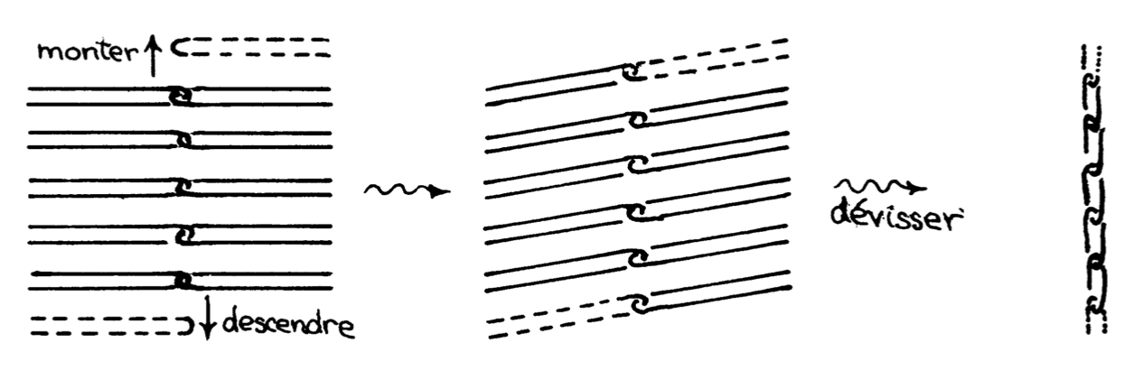
Figure 18.
By this lemma, one can shrink many decompositions related to Whitehead compacta. For example, let \( \mathcal{W}\subset \mathbb{R}^3 \) be a Whitehead compactum and let \[\mathcal{D}=\{t\in W\mid t\in [0,1], W\in \mathcal{W}\}\]
be the decomposition \( I\times \mathcal{W} \) of \( \mathbb{R}\times \mathbb{R}^3=\mathbb{R}^4 \). Then \( \mathcal{D} \) is shrinkable by Lemma 4.7 applied to the solid tori \( T \), \( T^{\prime} \), \( T^{\prime\prime} \), …whose intersection is \( \mathcal{W} \). Therefore \( \mathbb{R}^4/\mathcal{D} \) is homeomorphic to \( \mathbb{R}^4 \). Moreover, by Proposition 4.2 (localisation principle), we have that \[ (0,1)\times \mathbb{R}^3/\mathcal{W} \]
is homeomorphic to \( (0,1)\times \mathbb{R}^3 \). Hence we have the following celebrated fact.
This is a result of Andrews and Rubin [e16] in 1965, proved after analogous results, but more difficult, of Bing [e5] in 1959, which is a curious anachronism. There is a good explanation! A. Shapiro, at the time when he succeeded in turning \( S^2 \) inside out in \( S^3 \) by a regular homotopy, compare [e31], had also established Theorem 4.8. In any case, Bing tells me that D. Montgomery had communicated to him this claim without being able himself to justify it except by giving an easier argument (see Lemma 4.9) showing that \[ \mathbb{R}\times (S^3\smallsetminus \mathcal{W}) \]
is homeomorphic to \( \mathbb{R}^4 \), compare [e6]. Did the proof of Shapiro from the 50s disappear without a trace?
To establish the flatness of the discs \( \{E(\alpha)\} \) constructed in Section 3.9, we will also need a lemma that is easier than Lemma 4.7, treating again the Whitehead pair \( (T,T^{\prime}) \). Let \( D \) be a meridional disc of \( T \) that cuts \( T^{\prime} \) transversally in two discs.
and \( B\cap (\mathbb{R}\times D) \) is an equatorial 3-ball of the form \[ (\text{interval})\times D_0\subset \mathbb{R}\times D .\]
Proof of Lemma 4.9. This has nothing to do with the proof of Lemma 4.7! We find \( B \) easily from a 2-disc immersed in \( T \) like in Figure 20 (compare Section 3.9). ◻
To establish that \[ (B^2\times \mathring{D}^2)/\mathcal{D}_+ \]
is homeomorphic to \( B^2\times \mathring{D}^2 \), we will now use the construction of Section 3.
Proof of Proposition 4.10. We apply Theorem 4.4, Lemma 4.7 (or Lemma 4.9, without exploiting the last condition of Lemma 4.9). For this, it is convenient to remark first that for all open \( \mathcal{W} \)-saturated \( U \) in \( B^2\times D^2 \), \( W\cap U \) is contained in an open subset of \( U \) that is a disjoint union of open sets of the form \[ \mathring{I}^{\prime}\times \mathring{T}(a_1,\ldots,a_k) ,\]
where \( I^{\prime} \) is an interval. ◻
Our next goal is the flatness of the discs \[ E(\alpha)=q(D(\alpha))\subset (B^2\times \mathring{D}^2)/\mathcal{W}. \]
Let \[\mathcal{W}(\alpha)=\{w\in \mathcal{W}\mid w\cap D(\alpha)\neq \emptyset\},\]
and let \( W(\alpha)=\bigcup \mathcal{W}(\alpha) \).
Proof of Proposition 4.11. We apply Lemma 4.9 and the relative criteria (Theorem 4.4). For every open \( \mathcal{W}_\alpha \)-saturated \( U \) of \( B^2\times \mathring{D}^2 \), the intersection \( W_\alpha\cap U \) is trivially contained in an open set which, for some integer \( l \), is a disjoint union of open sets of the form \[ \mathring{I}^{\prime}\times \mathring{T}^{\prime}\subset U ,\]
where \( T^{\prime} \) is a connected component of multiple solid tori \( T_l(b_1,\ldots,b_l) \) and \( i^{\prime} \) is an interval.
Condition (d) of Section 3.9 allows us to choose these sets so that in addition, for each:
- \( D(\alpha)\cap (I^{\prime}\times T^{\prime}) \) is a single 2-disc, which is projected onto a meridional disc \( D \) of \( T^{\prime} \) which is also a connected component of \( D^{\prime}(\alpha)\cap T^{\prime} \); see Section 3.9.
By condition (b) of Section 3.9 the meridional disc \( D \) ideally chopped off \( T_{l+1/6}\cap T^{\prime} \), so Lemma 4.9 gives us disjoint 4-balls \( B_1,\ldots,B_s \) in \( \mathring{I}^{\prime}\times \mathring{T}^{\prime} \), such that
- each intersection \( B_i\cap D(\alpha) \) is a diametral 2-disc and not knotted in \( B_i \), and
- \( \mathring{B}_1\cup\cdots\cup \mathring{B}_s \) contains the compact
set
\[
W^+\cap (\mathring{I}^{\prime}\times \mathring{T}^{\prime})\supset W_\alpha\cap
(\mathring{I}^{\prime}\times \mathring{T^{\prime}}).
\]
For all compact \( K \) in \( \mathring{B}_i \) and all \( \epsilon > 0 \), we can easily find a homeomorphism \( h : B_i\to B_i \) with compact support which respects \( \mathring{B}_i\cap D(\alpha) \) and such that \( \operatorname{diam} h(K) < \epsilon \). The criteria of Theorem 4.4 (respecting \( D(\alpha) \)) is therefore satisfied. ◻
Proof of Proposition 4.12. The open set \[ U_\alpha=(B^2\times \mathring{D}^2)\smallsetminus (W_\alpha\cup D(\alpha)) \]
is clearly homeomorphic to \[ (B^2\times \mathring{D}^2)/\mathcal{W}_\alpha-q_\alpha(D(\alpha)) \]
by \( q_\alpha \). Therefore, by Propositions 4.2 and 4.3, the quotient map \[ q_\alpha^{\prime} : (B^2\times \mathring{D}^2)/\mathcal{W}_\alpha\to (B^2\times \mathring{D}^2)/\mathcal{W} \]
is approximable by homeomorphisms fixing \( q_\alpha^{\prime} \) on the flat disc \( q_\alpha(D(\alpha)) \). Therefore, \[ q(D(\alpha))=q^{\prime}(\alpha)\circ q(\alpha)(D(\alpha)) \]
is flat. ◻
We now propose to finish by showing that the quotient maps \begin{align*} B^2\times \mathring{D}^2 &\xrightarrow{\approx}(B^2\times \mathring{D}^2)/\mathcal{W}\\ &\xrightarrow{p_1}((B^2\times \mathring{D}^2)/\mathcal{W})/\{E(\alpha)\}\\ &\xrightarrow{p_2} (B^2\times \mathring{D}^2)/\mathcal{D}_+ \end{align*}
are approximable by homeomorphisms.
Proof of Proposition 4.13. This follows from Propositions 4.12, 4.6 and 4.5. ◻
To approximate \( p_2 \) by homeomorphisms, we need a little preparation. According to Propositions 4.13 and 4.10, there is a shrinking map \[ r : B^2\times\mathring{D}^2\to B^2\times \mathring{D}^2 \]
inducing the same decomposition as the quotient map \[ ((B^2\times \mathring{D}^2)/\mathcal{W})/\{E(\alpha)\} ;\]
we can identify the domain of \( p_2 \) with \( B^2\times \mathring{D}^2 \) by \( r \).
The decomposition \( \mathcal{P} \) constituted of the preimages \[ p_2^{-1}(y)=\{\text{a point}\} \]
is the countable collection of natural quotients of connected components of holes \( T_*(\alpha) \) and \( B_* \), which now identify \( r(T_*(\alpha)) \) and \[ r(B_*)\subset B^2\times \mathring{D}^2 .\]
We observe that \( \mathcal{P} \) is null. The quotient map \[ \lambda B^2\times \mu D^2=B_*\to rB_* \]
shrinks the Whitehead compactum \[ \mathcal{W}(\partial B_*)=\{w\in \mathcal{W}\mid w\subset B_*\}, \]
and these compact sets lie in \[ \lambda B^2\times \mu \partial D^2\subset \partial B_* .\]
This will result in the following proposition.
admits a bicollar neighbourhood.
Proof of Proposition 4.15. This is equivalent to the existence of a bicollar neighbourhood in \[ (\mathbb{R}\times \partial B_*)/(0\times \mathcal{W}(\partial B_*)) .\]
However, by (slightly generalised) Theorem 4.8 and Propositions 4.2 and 4.3, the quotient map of the latter space on \[ (\mathbb{R}\times \partial B_*)/(\mathbb{R}\times \mathcal{W}(\partial B_*)) \]
is approximable by homeomorphisms, fixing the quotient of \( 0\times \partial B_* \). ◻
Proof of Proposition 4.14. The map \( r \) factorises into \( r^{\prime\prime}\circ r^{\prime} \) where \( r^{\prime} \) factors through \( \mathcal{W}(\partial B_*) \). However, Proposition 4.15 ensures a bicollar neighbourhood of \( r^{\prime}(\partial B_*) \) in \[ (B^2\times \mathring{D}^2)/\mathcal{W}(\partial B_*) .\]
Propositions 4.2 and 4.3 ensure that \( r^{\prime\prime} \) is approximable by homeomorphisms fixing \( r^{\prime}(\partial B_*) \). Therefore, the pair \[ ((B^2\times \mathring{D}^2)/\mathcal{W}(\partial B_*), r^{\prime}(\partial B_*)) \]
(with the bicollar) is homeomorphic to \( (B^2\times \mathring{D}^2,r(\partial B_*)) \). ◻
Proof of Proposition 4.16. Given an open neighbourhood \( U \) of \( r(B_*) \), there exists, by Proposition 4.14, a homeomorphism \[ h : B^2\times \mathring{D}^2\to B^2\times \mathring{D}^2 \]
with compact support in a bicollar \( V \) of \( r(\partial B_*) \) in \( U \), such that \[ h(r(B_*))\subset r(\mathring{B}_*) .\]
Since \( r(\mathring{B}_*) \) is homeomorphic to \( \mathbb{R}^4 \), there exists a map \( g \) with support in \( r(\mathring{B}_*) \) and approximable by homeomorphisms such that \( g\circ h\circ r(B_*) \) is a point in \( r(\mathring{B}_*) \). Let \[ f=g\circ h : B^2\times \mathring{D}^2\to B^2\times \mathring{D}^2. \]
By uniform continuity on the compact support \( F\subset r(B_*)\cup V \) of \( f \), we know that, for a given \( \epsilon > 0 \), there exists \( \delta > 0 \) such that for all sets \[ E\subset B^2\times \mathring{D}^2 \]
of diameter less than \( \delta \), the diameter of \( f(E) \) is less than \( \epsilon \). By Lemma 4.17, there exists a stretch homeomorphism \( \theta : B^2\times \mathring{D}^2 \) fixing \( r(B_*) \) and with support in \( V \) such that, for all \( P\in \mathcal{P} \) distinct from \( B_* \) such that \[ \theta(P)\cap F\neq \emptyset ,\]
we have \( \operatorname{diam} \theta(P) < \delta \). Then \[ f=f_0\circ \theta \]
satisfies \( \mathcal{R}(B^2\times \mathring{D}^2,B_*;\mathcal{P}) \). ◻
such that \( \Phi=\varphi\times\operatorname{Id}_X \) satisfies that, for all \( E\in l \) such that \[ \Phi(E)\cap (X\times [0,1])\neq \emptyset, \]
we have \( \operatorname{diam}(\Phi(E)) < \epsilon \).
Proof of Lemma 4.17 (Indications.) Figure 21 completes the proof. □
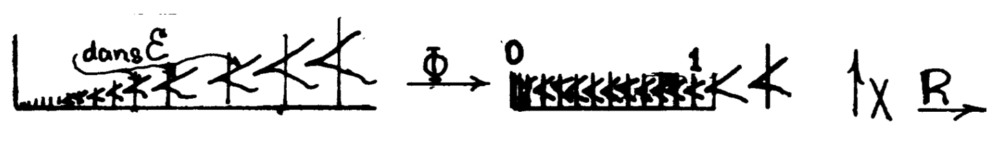
Figure 21.
All elements of \( \mathcal{P} \) distinct from \( r(B_*) \) are of the form \( r(T_*^{\prime}(\alpha)) \) where \( T_*^{\prime}(\alpha) \) is a connected component of a torus \( T_*(\alpha) \). Following the method of the proof of Proposition 4.16, we establish similarly the following proposition.
Proof of Proposition 4.18 (indications). The quotient of \[ T_*^{\prime}(\alpha)=J(\alpha)\times T^{\prime}(\alpha) ,\]
by the longitude \( l(\alpha) \) that is in \( D(\alpha) \), is a cone whose centre is the quotient of \( l(\alpha) \), and the base is a solid torus. \[ \delta r(T_*^{\prime}(\alpha))-r(l(\alpha)) \]
has a bicollar neighbourhood in \( B^2\times \mathring{D}^2 \), compare Proposition 4.13. The accumulation points of elements \( P\neq \text{a point} \) of \( \mathcal{P} \) are the centre \( r(l(\alpha)) \) and a compact set \[ r(W\cap \partial T_*^{\prime}(\alpha)) \]
far from \( r(l(\alpha)) \). ◻
Proof. Apply Propositions 4.18, 4.16 and 4.5. ◻
5. Freedman’s approximation theorem
is nowhere dense and at most countable. Then, \( f \) can be approximated by homeomorphisms.
In the case that \( S(f) \) is finite, this theorem is well known since it constitutes the essential part of the celebrated Schönflies theorem which was established around 1960 by B. Mazur, M. Brown and M. Morse.
Recall that a compact set \( A \) in a topological \( n \)-manifold \( M \) (without boundary) is cellular if each neighbourhood of \( A \) contains a neighbourhood which is homeomorphic to \( B^n \).
Compare the Bing shrinking criterion, Theorem 4.1 [e8]. A direct proof shrinks \( A \) gradually to a point.
Proof of Theorem 5.1 if \( S(f) \) is a point. Let \( y_0=S(f) \) and \( A=f^{-1}(y_0) \), we have that \( X\smallsetminus A \) is homeomorphic to \( \mathbb{R}^n \). Since \( X \) is homeomorphic to \( S^n \), it follows that \( A \) is cellular in \( X \) (exercise). Then, we obtain approximations by applying Lemma 5.2. ◻
In the setting of Freedman’s ideas, the case where \( S(f) \) is \( n \) points, \( n\geq 2 \), is already as difficult as Theorem 5.1. However one can consult [e8], [e10] for an easy proof. We recall the Schönflies theorem.
Then the closure of each of the two components of \( S^{n}-\Sigma \) is homeomorphic to the \( n \)-ball \( B^n \).
Proof of Theorem 5.3 (starting from Theorem 5.1 for \( S(f) \) consisting of two points). Let \( X_1 \) and \( X_2 \) be two connected components of \( S^n\smallsetminus \mathring{N} \) and \( W_1 \) and \( W_2 \) be the closures of connected components of \( S^n\smallsetminus \Sigma^{n-1} \) containing \( X_1 \) and \( X_2 \), respectively. It is necessary to show that \( W_1 \) and \( W_2 \) are homeomorphic to \( B^n \).
Shrinking \( X_1 \) and \( X_2 \), we obtain a quotient map \[f : S^n\to S^n/\{X_1,X_2\}\approx (\Sigma\times [-1,1])/\{\Sigma\times 0,\Sigma\times 1\}\approx S^n\]
that is approximable by homeomorphisms from Theorem 5.1 (the case of \( S(f) \) is two points). So \( X_1 \) and \( X_2 \) are cellular in \( S^n \). Apply Lemma 5.2 to \( X_i\subset \mathring{W}_i \), we deduce that \[W_i\to W_i/X_i\approx \Sigma\times [0,1]/\{\Sigma\times 1\} \approx B^n\]
is approximable by homeomorphisms. ◻
To prove Theorem 5.1, Freedman introduced a nice trick of iterated replication of the approximation map, which vaguely reminds me of the arguments of Mazur [e7]. This trick leads us to leave the category of continuous maps and to instead work in the less familiar realm of closed relations. It was during the seventies that closed relations imposed themselves for the first time on geometric topology; they surfaced implicitly in a very original article by M. A. Stanko [e24] and have become essential since: I believe that it would be a herculean task to prove, without closed relations, the subsequent theorem of Ancel and Cannon [e30] that any topological embedding \( S^{n-1}\to S^n \), \( n\geq 5 \), can be approximated by locally flat embeddings.
which is also closed if \( Y \) is compact. Therefore the collection of closed relations between compact spaces is a category.
A continuous map \( f : X\to Y \) gives a closed relation \[ \{(x,f(x))\mid x\in X\} \]
(the graph of \( f \)) which we still call \( f \). Reciprocally, provided that \( Y \) is compact, a closed relation \( R : X\to Y \) is the graph of a continuous function (which is uniquely determined) if \( R\cap x\times Y \) is a point for all \( x\in X \).
By extending usual notions for continuous functions, for \( A\subset X \) and \( B\subset Y \), we have
- the image \( R(A)=\{y\in Y\mid \text{there exists }x\in A\text{ such that }(x,y)\in R\} \),
- the restriction \( R|_{A} : A\to Y \) is the closed subset \( R\cap A\times Y \) in \( A\times Y \),
- the inverse \( R^{-1} : Y\to X \) such that \( \{(y,x)\in Y\times X\mid (x,y)\in R\} \).
To exploit an analogy between a function \( X\to Y \) and a relation \( R : X\to Y \), we will at any time assimilate \( R \) to the function that associates for each point \( x\in X \) to a subset \( R(x)\subset Y \).
Proof of Theorem 5.1. Any submanifold of codimension 0 that is introduced will be assumed to be topological and locally flat. Let \( N \) be a neighbourhood of \( f \) in \( X\times Y \). The theorem asserts that there exists a homeomorphism \( H : X\to Y \) such that \( H\subset N \).
By removing a small \( n \)-ball \( D\subset Y\smallsetminus\overline{S(f)} \) from \( Y \) and removing its preimage \( f^{-1}(D) \) from \( X \), we see that it is permissible to adopt the following.
is nowhere dense and at most countable and \( S(f)\subset \operatorname{Int} Y \). Then \( f \) can be approximated by homeomorphisms.
It is easy to see that Theorem 5.4 implies Theorem 5.1 using the special case of Theorem 5.3 (Schönflies theorem) where \( \Sigma^{n-1} \) bounds a ball (see observation after Theorem 5.3).
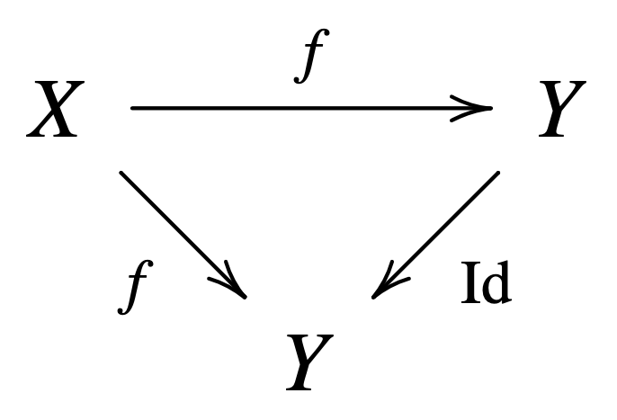
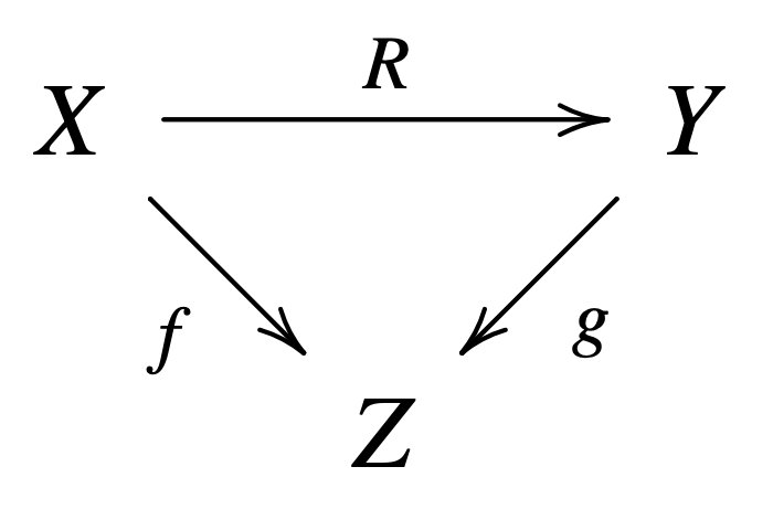
The first step of an inductive construction of \( H \) is to apply the following proposition to the triangle shown to the right. Moreover, the neighbourhood \( N \) of Proposition 5.5 becomes \( N \) the above; and \( L \) becomes \( Y \).
Suppose that \( X \) and \( Y \) are homeomorphic to \( B^n \). A relation \( R : X\to Y \) is called good if it is closed, and satisfying the following conditions:
- \( R\subset X\times Y \) projects onto \( X \) and onto \( Y \).
- \( R(x) \) is not a singleton set for at most countably many points in \( X \) and these exceptional points constitute a nowhere dense set contained in \( \operatorname{Int} X \). The same holds for \( R^{-1} \).
It is said that a good relation \( R^{\prime} : X\to Y \) is finer than \( R \) if \[ R^{\prime}\subset R\subset X\times Y .\]
- \( R\subset (f^{-1}(\overline{L})\times g^{-1}(\overline{L}))\cup (f^{-1}(Z\smallsetminus L)\times g^{-1}(Z\smallsetminus L)) \); it is inevitable if the triangle switches.
- \( R=g^{-1}\circ f \) on \( f^{-1}(\overline{L}) \).
- \( R \) is given by the intersection graph of a homeomorphism
\[ f^{-1}(Z\smallsetminus L)\to g^{-1}(Z\smallsetminus L) .\]
- The singular sets \( S(f) \) and \( S(g) \) are separated on \( L \), that is, there are two open disjoint sets \( U \) and \( V \) which contain \( S(f)\cap L \) and \( S(g)\cap L \), respectively.
Then, for all \( \epsilon > 0 \), we can modify the three data \( g \), \( R \), \( L \) to \( g_* \), \( R_* \), \( L_* \) so that in addition to the same conditions above (with \( g_* \), \( R_* \), \( L_* \) instead of \( g \), \( R \), \( L \)), we have \( R_*=R \) on \( f^{-1}(Z\smallsetminus L) \), \( L_*\subset L \), and for all \( y\in Y \), \( \operatorname{diam} R_*^{-1}(y) < \epsilon \).
for all \( y\in Y \).
Proof of Addendum. If the conclusion is false, then there are two sequences of points of \( X\times Y \), say \( (x_k,y_k) \), \( (x_k,y_k^{\prime}) \), \( k=1,2,3,\dots \), which converge in compact \( R_* \) and such that \( d(y_k,y_k^{\prime})\geq \epsilon \). By compactness of \( X\times Y \), we can arrange that the sequences \( x_k \), \( y_k \) and \( y_k^{\prime} \) converge to \( x \), \( y \) and \( y^{\prime} \), respectively. Then, \( (x,y) \) and \( (x,y^{\prime}) \) belong to compact \( R_* \), but \( d(y,y^{\prime})\geq \epsilon \), which is a contradiction. ◻
Proposition 5.5 (with Addendum) will be used as a machine that swallows the data \( f \), \( g \), \( R \), \( L \), \( N \), \( \epsilon \) and manufactures \( f \), \( g_* \), \( R_* \), \( L_* \), \( N_* \).
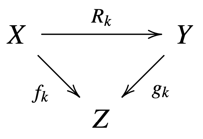
Let us continue constructing the homeomorphism \( H \), assuming Proposition 5.5. For \( k\geq 1 \), the \( k \)-th step constructs a triangle shown to the right (where \( Z \) is a copy of \( Y \)); a submanifold \( L_k\subset Z \) and a neighbourhood \( N_k \) of \( R_k \) in \( X\times Y \) such that \( f_k \), \( g_k \), \( R_k \), \( L_k \), \( N_k \) satisfy the conditions imposed on \( f \), \( g \), \( R \), \( L \), \( N \) in Proposition 5.5. The first step is already specified: Proposition 5.5 creates \( f_1 \), \( g_1 \), \( R_1 \), \( L_1 \), \( N_1 \) from \( f \), \( \operatorname{Id} \), \( f \), \( Y \), \( N \), 1.
Suppose that the \( k \)-th triangle is constructed and we construct the \( (k+1) \)-th triangle.
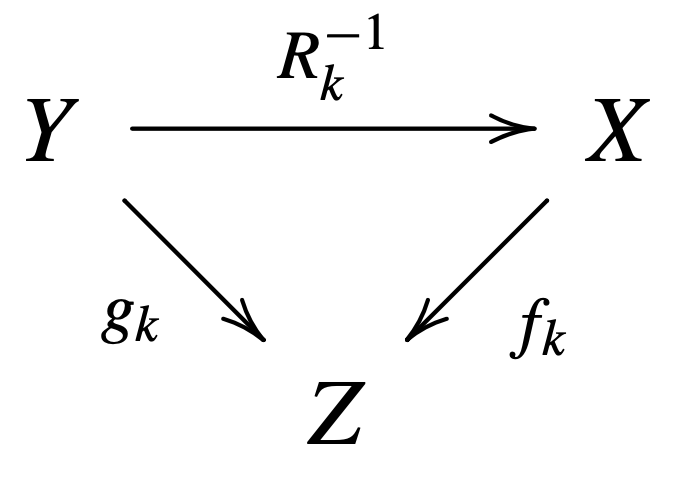
- If \( k \) is odd, then Proposition 5.5 gives \( g_{k+1} \), \( f_{k+1} \), \( R_{k+1}^{-1} \), \( L_{k+1} \), \( N_{k+1}^{-1} \) from \( g_k \), \( f_k \), \( R_{k}^{-1} \), \( L_k \), \( N_k^{-1} \), \( 1/k \). In brief, we apply Proposition 5.5 to the reverse triangle shown to the right.
- If \( k \) is even, then it is same as the first step: Proposition 5.5 gives \( f_{k+1} \), \( g_{k+1} \), \( R_{k+1} \), \( L_{k+1} \), \( N_{k+1} \) from \( f_k \), \( g_k \), \( R_k \), \( L_k \), \( N_k \), \( 1/k \).
By induction, we have \( N\supset N_1\supset N_2\supset \cdots \). We define \( H=\bigcap_k N_k \). Then, \( H \) is a homeomorphism since, for all \( x \), we have \[ \operatorname{diam} H(x)\leq \operatorname{diam} N_k(x)\leq 1/k, \]
for all even \( k \), and \[ \operatorname{diam} H^{-1}(x)\leq \operatorname{diam} N_k^{-1}(x)\leq 1/k, \]
for all odd \( k \). This homeomorphism \( H \) in the neighbourhood \( N \) of \( f \) completes the proof of Theorem 5.1 assuming Proposition 5.5. ◻
Proof of Proposition 5.5. To explain the essential idea of Freedman, the reader should read the proof with a view to (re)proving that a surjection \( f : B^n\to B^n \) such that \[ S(f)=\{\text{a point}\}\subset \operatorname{Int} B^n \]
is approximable by homeomorphisms (for this, we set \( f=R \) and \( g=\operatorname{Id} \)). Then, it should be noted that as soon as \[ S(f)=\{k\text{ points}\}\subset \operatorname{Int} B^n, \]
the same argument leads us to approximate \( f \) by relations which crush nothing, but which blow up \( k(k-1) \) points.
Consider the preimages \( R^{-1}(y) \), \( y\in Y \), of diameter \( \geq \epsilon \), that we want to eliminate. According to (a), (b) and (c), these sets constitute the preimage by \( f \) of the set \( (S_\epsilon(f)\cap L)\subset Z \), where \[ S_\epsilon(f)=\{z\in Z\mid \operatorname{diam}f^{-1}(z)\geq \epsilon\}, \]
which will allow us to follow the case in \( Z \). Note that \( S_\epsilon(f) \) is compact although, typically, \( S(f) \) is not. For example, \( S_\epsilon(f) \) is finite in the case of interest to Freedman (see Section 4).
Proof of Lemma 5.6 Consider the space \( \operatorname{Aut}(M,\partial M) \) of automorphisms of \( M \) fixing \( \partial M \), provided with the complete metric \[ \operatorname{sup}(d(f,g),d(f^{-1},g^{-1})) \]
where \( d \) is the uniform convergence metric. In \( \operatorname{Aut}(M,\partial M) \), the set of automorphisms \( \theta \), such that the first \( k \) points \( A_k \) of \( A \) and \( B_k \) of \( B \) satisfying \[ \theta(A_k)\cap \overline{B}=\emptyset=\theta(\bar{A})\cap B_k, \]
constitute an open subset \[ U_k\subset \operatorname{Aut}(M,\partial M) \]
everywhere dense in \( \operatorname{Aut}(M,\partial M) \), because \( \bar{A} \) and \( \overline{B} \) are closed, nowhere dense in \( M \).
Then, the famous Baire category theorem asserts that the countable intersection \( \bigcap_k U_k \) is everywhere dense in \( \operatorname{Aut}(M, \partial M) \). Note that \( \bigcap_k U_k \) is the set of \( \theta \) in \( \operatorname{Aut}(M,\partial M) \) such that \[ \theta(A)\cap \overline{B}=\emptyset =\theta(\bar{A})\cap B. \]
But, for \( X_1 \), \( X_2 \) in a metrisable \( M \), the condition that \[ X_1\cap \overline{X}_2=\emptyset =\overline{X}_1\cap X_2 \]
leads to the separation of \( X_1 \) and \( X_2 \) in \( M \). In effect, seen in the open subset \( M\smallsetminus (\overline{X}_1\cap \overline{X}_2) \) of \( M \), the sets \[ \overline{X}_1\smallsetminus (\overline{X}_1\cap \overline{X}_2) \quad\text{and}\quad (\overline{X}_1\cap \overline{X}_2) \]
are always disjoint, closed and hence separated. The mentioned condition ensures that they contain respectively \( X_1 \) and \( X_2 \). ◻
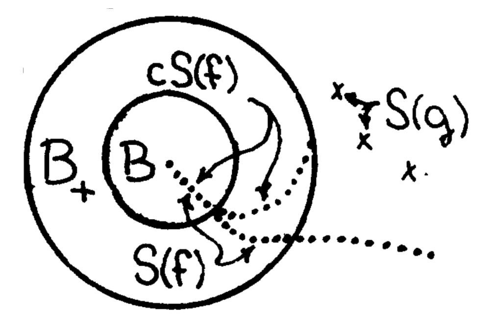
- \( S_\epsilon(f)\cap L\subset \mathring{B}_+ \).
- \( S(g)\cap B_+=\emptyset \).
- Each connected component \( B_+^{\prime} \) of \( B_+ \) is small in the sense
that
\[
(f^{-1}(B_+^{\prime}))\times (g^{-1}(B_+^{\prime}))\subset N,
\]
and standard in the sense that \( Z\smallsetminus \operatorname{Int}B_+^{\prime} \) is homeomorphic to \( S^{n-1}\times [0,1] \).
Proof of Claim 5.7. Identify \( Z \) with \( B^n\subset \mathbb{R}^n \) to give \( L \) an affine linear structure. Let \( K \) be a compact neighbourhood of the compact set \( S_\epsilon(f)\cap L \) which is a subpolyhedra of \( L \) and disjoint from \( S(g) \), see Proposition 5.5(c). We subdivide \( K \) into a simplicial complex of which each simplex \( \mathcal{L} \) is linear in \( L \) and so small such that \[ f^{-1}(\Delta)\cap g^{-1}(\Delta)\subset N. \]
Then (compare, the proof of Lemma 5.6), by a small perturbation (a translation if we want) of \( K \) in \( L \), we disengage the \( (n{-}1) \)-skeleton \( K^{(n-1)} \) from the compact countable \( S_\epsilon(f) \), without harming the properties of \( K \) already established. Finally, \( B_+ \) is defined as \( K \) minus a small \( \delta \) open neighbourhood of \( K^{(n-1)} \) in \( \mathbb{R}^n \). Each component \( B_+^{\prime} \) of \( B_+ \) is convex and in \( \operatorname{Int} Z=\mathring{B}^n \); therefore \( Z\smallsetminus \mathring{B}_+^{\prime} \) is homeomorphic to \( S^{n-1}\times [0,1] \), by an elementary argument. ◻
In \( \operatorname{Int} B_+ \), we choose now a union \( B \) of balls (one in each connected component of \( B_+ \)), which still satisfies (1), (2), (3) and also
(4) \( S(f)\cap \partial B=\emptyset \).
We set \( L_*=L\smallsetminus B \). For each connected component \( B_+^{\prime} \) of \( B_+ \), we are now modifying \( g \) and \( R \) above \( B_+^{\prime} \) to define \( g_* \) and \( R_* \). These changes for the various connected components \( B_+^{\prime} \) are disjoint and independent. Therefore, it is enough to specify one. Moreover, in order to simplify the notation, we allow ourselves to specify this change only in the case that \( B_+ \) is connected.
Let \( c : Z\to B_+ \) be a homeomorphism, called the compression, which fixes all points of \( B \). (We remember that \( Z\smallsetminus \mathring{B} \) is homeomorphic to \[ S^{n-1}\times [0,1] \]
and \( B_+\smallsetminus \mathring{B} \).) We should modify \( c \) by composing with a homeomorphism \( \theta \) of \( B_+\smallsetminus \mathring{B} \) fixing \[ \partial B_+\cup \partial B \]
given by Lemma 5.6, to assure that \( S(f) \) and \( c(S(f)) \) are separated on the open \( \mathring{B}_+\smallsetminus B \).
Since \( g^{-1}(B_+) \) is a ball in \( Y \) (in fact, \( g \) is a homeomorphism over \( B_+ \)), we can also choose \( i \) so that \( i|_{\partial X} \) is \[ (g^{-1}\circ c\circ f)|_{\partial X} .\]
We set \[g_*=\begin{cases}g&\mbox{on }g^{-1}(Z\smallsetminus \mathring{B}_+),\\ c\circ f\circ i^{-1}&\mbox{on }g^{-1}(B_+).\end{cases}\]
On \( g^{-1}(\partial B_+) \), \( g_* \) is well-defined since \[ g=c\circ f\circ (g^{-1}\circ c\circ f)^{-1} \]
on \( g^{-1}(\partial B_+) \). We set \[R_*=\begin{cases}R&\mbox{on }f^{-1}(Z\smallsetminus \mathring{B}_+),\\ g^{-1}\circ f=(i\circ f^{-1}\circ c^{-1})\circ f&\mbox{on }f^{-1}(B_+).\end{cases}\]
More precisely, on \( f^{-1}(B_+) \), we specify \[R_*=\begin{cases}(i\circ f^{-1}\circ c^{-1})\circ f &\mbox{on }f^{-1}(B_+-\mathring{B}),\\ i&\mbox{on }f^{-1}(B). \end{cases}\]
On \( f^{-1}(\partial B) \), \( R_* \) is well-defined since \( c \) fixes all points of \( \partial B \), and \[ S(f)\cap \partial B=\emptyset .\]
We have now specified the modification \( L_* \), \( g_* \), \( R_* \) of \( L \), \( g \), \( R \) claimed by Proposition 5.5. (We remark that if \( B_+ \) is a union of \( k \) balls, rather than one ball, the modification is done in \( k \) disjoint and independent steps, each similar to the one just specified for connected \( B_+ \).)
Verifying the claimed properties for \( L_* \), \( g_* \), \( R_* \) is direct. (There are already manuscripts [1], [2] which offer more details.) ◻
We form \( \gamma_* \) of \( \varphi\sqcup \gamma_0 \) by identifying, via \( c|_{\partial Z} \), the subfibres (whose fibres are points) \( \varphi|_{\partial Z} \) and \( \gamma_0|_{\partial B_+} \). Then, we can identify the total space and the base of \[ \gamma_*=\varphi\cup \gamma_0 \]
to those of \( \gamma \) by an extension of \( \gamma_0\to \gamma \). More precisely, we use \[ (\operatorname{Id}|_{Z\smallsetminus \mathring{B}_+})\cup c \]
between bases, which is the identity on \( B\subset B_+ \). Then, \[ \varphi \quad\text{and}\quad \gamma_* : Y\xrightarrow{g_*}Z \]
are fibrations over \( Z \) naturally isomorphic on \( B\cup L \), which defines a relation \( R_* \) finer than the simple correspondence of fibres \( g_*^{-1}\circ f \).
Thus, as fibres, \( f_\infty \) and \( g_\infty \) are isomorphic. Moreover, each fibre of \( f_\infty \) or \( g_\infty \) is homeomorphic to a fibre of \( f \). I point out that \( f_\infty \) and \( g_\infty \) remind me of the two infinite products of Mazur [e7] and that \( H \) reminds me of the famous Eilenberg–Mazur swindle, which completes the proof of Theorem 5.3 (weakened version) given in [e7].
