| [letterhead] | |
| Yale University | |
| New Haven, Connecticut 06520 | |
| [letterhead] | |
| Department of Mathematics | |
| 12 Hillhouse Avenue | |
| Box 2155 Yale Station | |
| [handwriting] March 12, ’87 |
Dear Yves,
I attach a copy of what I wrote about wavelets with compact support. It is not (yet) an article: rather the sort of thing that I write for myself before writing an article, to let ideas crystallize. All the proofs are there.
I was telling you on the phone that my way of seeing wavelets with compact support was more graphical. That is also the way I came upon them. At the start, fix \( f(n), \) \( g(n). \) (In fact, Bob Hummel, one of the researchers on [computer] vision at NYU, gave me some articles, including one by J. Burt, which contains a decomposition and recomposition using a single filter. It is not a decomposition using wavelets, and the algorithm proposed by S[téphane] Mallat is not only nicer but also more efficient. Stéphane refers to Burt (Laplacian pyramid schemes) in his paper. Since I’d read Burt a few days before receiving Stéphane’s paper, I was in just the right frame of mind to take the filters, or the discrete algorithm, as a starting point rather than as a consequence of the (beautiful!) “wavelets + multiscale” structure.) So then, fix the functions \( f(n) \) and \( g(n). \)
Reading Stéphane’s article, I immediately realized that the discrete algorithm rests completely on \begin{align} \label{1} &\sum_k\,\bigl[f(n-2k)f(m-2k)+g(n-2k)g(m-2k)\bigr]=\delta_{mn} \\ \label{2} \hbox{and}\quad& \sum_k\,\bigl[f(n-2k)g(n-2l)\bigr]=0. \end{align}
So I asked myself if there exist \( f(n), \) \( g(n) \) satisfying those conditions and not necessarily coming from a wavelet basis. And in fact they do exist. One example is \begin{align*} f(0)&=\lambda\mu N^{-1},& f(1)&=\lambda N^{-1},& f(2)&= N^{-1},& f(3)&= -\mu N^{-1},\\ g(0)&=\mu N^{-1},& g(1)&=N^{-1},& g(2)&=-\lambda N^{-1},& g(3)&= \lambda \mu N^{-1},\\ \end{align*}
where \( N=[(1+\lambda^2)(1+\mu^2)]^{1/2} \) and \( \lambda,\mu\in\mathbb{R} \) are arbitrary.
Since we like filters with finitely many “taps”, that is, with a finite number of nonzero coefficients \( f(n), \) I imposed that condition from the start as well.
The folks who play with those filters also like to have a certain kind of continuity. This is how they see the matter:
Let’s decompose a sequence \( c=(c_n)_{n\in \mathbb Z} \), which we imagine as a discrete signal, with a very small “step” between consecutive impulses. The decomposition, according to Stéphane’s algorithm, gives sequences \[ d_1=Gc, \quad d_2 = GFc,\quad \dots,\quad d_N=GF^{N-1}C\quad\hbox{and}\quad c_N=F^Nc, \]
where \[ (Gc)_k=\sum_n g(n-2k)c_n,\quad (Fc)_k=\sum_n f(n-2k)c_n \]
(in Stéphane’s notation), where each \( d_j \) has a “step” \( 2^j \) times larger than the initial \( c \), and \( c_N \) has a “step” \( 2^N \) times larger.
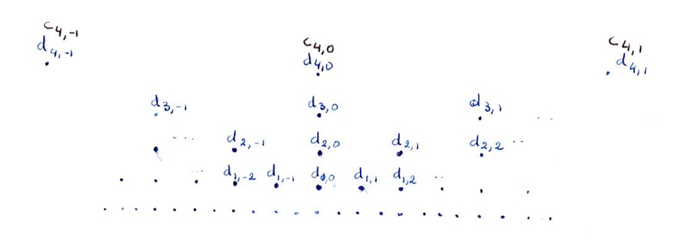
Let’s record all this in a pyramidal structure (the same drawings you use! I was very excited to find them in papers by engineers).
I’ll draw the \( d_j \) in blue and the final \( c_N \) in black.

For the reconstruction, we play a sort of videogame, which at each step sets down a series of numbers in black one row above the last black row from the previous turn. (I know that all this is much more familiar to you than to me, and that you’ll probably find my way of presenting it childish… But I really like this videogame image.) And the rule is, of course, \[ c_{n-1,k}=\sum_l (f(k-2l) c_{n,l}+g(k-2l) d_{n,l}). \]
What is new in Stéphane’s algorithm is that he uses two sequences \( f(n), \) \( g(n), \) which of course makes all the difference, compared with previous procedures!
The “continuity” that engineers like in this kind of videogame is the following. Suppose we take as given a single black “1”, at a fairly high level, and set all the \( d_j\equiv 0. \) The simplest initial conditions, if you wish. Then the reconstruction game gives me a series of increasingly detailed histograms.
For example: \[ f(-2)=f(2)=0.1, \quad f(-1)=f(1)=0.5, \quad f(0)=0.8. \]
(This \( f \) does not match \eqref{1} + \eqref{2}, but it is a filter that Burt uses.)
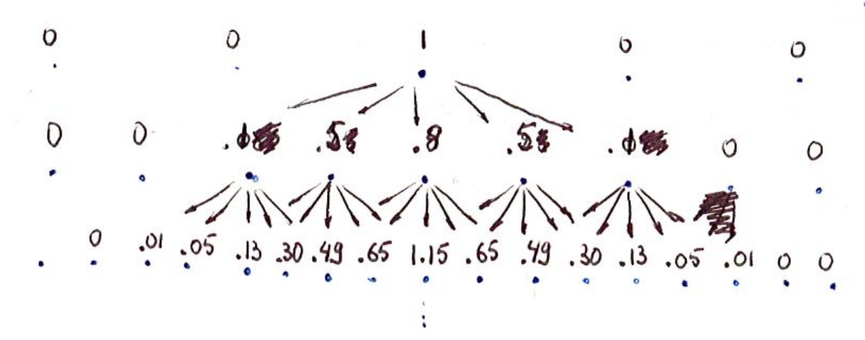
Or, more graphically:

What I was looking for, then, were solutions to \eqref{1} + \eqref{2} such that repeated application of \( F \) to the sequence \( (c_N)_k=\delta_{k0} \) leads to a continuous function. Or, more precisely, defining \[ (Th)(x)=\frac{2}{\sum f(n)}\sum\, f(n)\,h(2x-n), \]
I want \( T^n \chi_{[-1/2,1/2]} \) to converge to a continuous function as \( n \to\infty \). And in analyzing this convergence, I of course kept running into infinite products, and I manipulated the function that you denote by \( m_0 \) (which is \( F \) in Stéphane’s paper and \( \mathcal{F} \) in my notes. I’m sorry for the conflicting notation. I didn’t become aware of \( m_0 \) until the arrival of Thierry [Paul], who gave me copies of your recent articles.) By imposing certain conditions on \( \mathcal{F}(\xi)=\sum_n f(n)e^{in\xi}, \) which essentially amount to requiring that \( \mathcal{F} \) be divisible by \( (1+e^{i\xi})^n, \) I managed to prove in my notes that the \( T^n \chi_{[-1/2,1/2]} \) converge in \( L^2 \) — but one can also prove pointwise convergence — to a continuous function \( \phi \). The diagram immediately shows that \( |\mathrm{supp}\,\phi| < \infty \) if only a finite number of \( f(n) \) are nonzero. This “videogame” is also an easily programmable way to obtain a graph of \( \phi. \)
On the other hand, I realized that \eqref{1} + \eqref{2} imply \[ \sum_n f(n-2k)f(n-2l)=\delta_{kl} , \]
which is to say, that passing from one row of the videogame to the next preserves orthogonality in \( \ell^2. \) That is, the functions \( \phi(x) \) and \( \phi(x-k), \) obtained from the sequences \( (c)_n=\delta_{n0} \) and \( (\tilde c)_n=\delta_{nk}, \) are automatically orthogonal, because \( c \) and \( \tilde c \) are! (It was this fact, which I had already reached before but then lost sight of, that I recovered between my second and third letters: at one time I was afraid of being left only with frames, but with argument gave me back the bases that I announced to you in my first letter.)
The “frame” aspect came from the fact that \[ \sum_k c_{n-1,k}^2=\sum_j (c_{n,j}^2+d_{n,j}^2), \]
which is a consequence of \eqref{1} + \eqref{2}.
After my first letter I’d abandoned Toeplitz matrices and switched instead to complex functions, that is, \[ \mathcal{F}(\xi)=\frac{1}{\sum f(n)}\bigl(\alpha(2\xi)+e^{i\xi}\beta(2\xi)\bigr), \]
where \[\alpha(\xi)=\sum \,a(n) e^{in\xi}, \quad \beta(\xi)=\sum \,b(n) e^{in\xi}, \quad a(n)=f(2n), \quad b(n)=f(2n+1). \]
Then \eqref{1} + \eqref{2} reduce to \[ |\alpha(\xi)|^2+ |\beta(\xi)|^2=1 . \]
Since I’d been excited right away, while reading Stéphane’s article, by the possibility of construction other filters, not necessarily linked to wavelets (but they took their revenge!), I hadn’t paid much attention to the condition \[ |F(\xi)|^2+ |F(\xi+\pi)|^2=1 , \]
and, after my speed reading, I even thought that this condition was associated to the symmetry of \( \phi. \) When I met Stéphane he told me that that’s not the case, and I realized that my condition on \( \alpha \) and \( \beta \) was in fact identical to this one. And of course, I read your paper afterwards, and understood to what point all of this was inevitable.
Later I constructed examples that yield functions \( \phi\in C^k, \) \( k \) arbitrary (§4.3 in the attached notes). Since my examples had a support that grew exponentially with \( k, \) which I did not like at all, I tried to call you to find out how yours grew. I wasn’t able to reach you, but Alex [Grossman] told me over the phone that you obtained examples by iteration (that revelation blew me away, and right after hanging up with Alex I calculated that the growth would be less), and also that a result that I had finally proved after much thinking, about square roots of certain trigonometric polynomials, could be found in Pólya and Szegö. — The next day, since I found the iterative examples so much nicer than mine, I called you to propose to write a joint article.
I have not yet seen what you sent me at Courant, and I don’t know if it will have arrived by this weekend. But, you see, I like that graphical way of visualizing things. If I understood you correctly, in the manuscript you sent me you have incorporated compactly supported wavelets into the general framework of multiscale analysis. I see how they fall into place there naturally, but I wonder if the “graphical” approach (which is not as well-suited to other wavelets, in particular the “historical” wavelet), isn’t more intuitive as a way to see that compactly supported wavelets can exist. You see, I’ve become attached to that way of seeing things, which is the way I arrived at them.
An experience I had a few years ago might help explain this sense of attachment. Here is how it happened. When I was at Princeton, I worked with Elliott Lieb on a problem connected to the stability of matter, and we obtained a nice result. Since it was a problem that Elliott gave me, and since we had discussed it together a lot, and he had suggested some key ideas, I wrote the article, after having proved everything we wanted, and of course I put both of our names on it. Reading the article, Elliott thought that the proofs were accurate, correct, but not very nice. So he found a much nicer way of proving the same result, with better constants, and I rewrote the article with the new proofs. Those things happen, that’s life, and Elliott’s reaction was perfectly correct (and we’ve published joint papers since), but I have always felt that the second version, where the proofs, though put on paper by me, visibly bear the Lieb brand, had nothing to do with me, that it wasn’t really my paper, that I had no merit in it. I still have “my” version in some drawer in Brussels. — And so I am a bit afraid that I might be in a similar situation now. Since my relationship with you is much warmer than with Elliott (and I’m very grateful for that!), I thought I’d try to explain it. At the same time, I understand that you prefer a global presentation, where all wavelets fit, and where compactly supported wavelets have their little ecological niche in the great forest of wavelets. But I have not made any contribution to that view, although of course I admire it a lot. On the other hand, I like my videogame idea… So perhaps, as you were saying, there is some point in writing separate texts. — But we will talk about all this in Paris. I hope I haven’t bored you too much with these “considerations”…
See you soon! Hugs for everyone.
Ingrid
\[ \star\qquad\star\qquad\star \]
Cher Yves,
Ci-joint je t’envoie une copie de ce que j’ai rédigé sur les ondelettes à support compact. Il ne s’agit pas (encore) d’un article: c’est plutôt le genre de chose que je rédige pour moi-même avant d’écrire un article, afin de me clarifier les idées. Toutes les démonstrations y sont.
Je te disais, au téléphone, que ma façon de voir les ondelettes à support compact était plus graphique. C’est aussi la façon dont je les ai trouvées. Au départ, soient \( f(n), \) \( g(n). \) (En fait, Bob Hummel, qui fait “de la vision” à NYU, m’avait passé des articles, notamment de J. Burt, où il a une décomposition \( + \) reconstruction avec 1 seul filtre. Il ne s’agit pas d’une décomposition utilisant des ondelettes, et l’algorithme proposé par S. Mallat est non seulement joli, mais aussi plus efficace. Stéphane réfère à Burt (Laplacian pyramid schemes) dans son papier. Comme j’avais lu Burt quelques jours avant de recevoir le papier de Stéphane, j’étais tout à fait dans le “frame of mind” pour prendre les filtres, ou l’algorithme discret, comme point de départ plutôt que comme conséquence de la (très belle!) structure ondelettes \( + \) multiscale.) Donc, soient \( f(n), \) \( g(n). \)
En lisant l’article de Stéphane, je me suis tout de suite rendu compte que l’algorithme discret reposait complètement sur \begin{align} \label{3}\tag{1} &\sum_k\,\bigl[f(n-2k)f(m-2k)+g(n-2k)g(m-2k)\bigr]=\delta_{mn} \\ \label{4}\tag{2} \hbox{et}\quad& \sum_k\,\bigl[f(n-2k)g(n-2l)\bigr]=0. \end{align}
Et je me suis alors demandée s’il existait des \( f(n), \) \( g(n) \) satisfaisant ces conditions, et qui ne seraient pas nécessairement dérivés d’une base d’ondelettes. Et, en fait, il en existe. Un exemple est \begin{align*} f(0)&=\lambda\mu N^{-1},& f(1)&=\lambda N^{-1},& f(2)&= N^{-1},& f(3)&= -\mu N^{-1},\\ g(0)&=\mu N^{-1},& g(1)&=N^{-1},& g(2)&=-\lambda N^{-1},& g(3)&= \lambda \mu N^{-1},\\ \end{align*}
où \( N=[(1+\lambda^2)(1+\mu^2)]^{1/2} \) et \( \lambda,\mu\in\mathbb{R} \) arbitraires.
Comme on aime les filtres avec “a finite number of taps”, c.à.d avec un nombre fini de coefficients \( f(n)\neq 0, \) j’imposais cette condition dès le départ aussi.
Les gens que jouent avec des filtres aiment avoir une certain continuité aussi. Leur façon de voir est la suivante.
Décomposons une séquence \( c=(c_n)_{n\in \mathbb Z} \), que nous imaginons être un signal discet, avec un “pas”, entre deux impulsions consécutives, très petit. La décomposition, selon l’algorithme de Stéphane, donne des séquences \[ d_1=Gc, \quad d_2 = GFc,\quad \dots,\quad d_N=GF^{N-1}C\quad\hbox{et}\quad c_N=F^Nc, \]
où \[ (Gc)_k=\sum_n g(n-2k)c_n,\quad (Fc)_k=\sum_n f(n-2k)c_n \]
(notations de Stéphane) où chaque \( d_j \) a un “pas” \( 2^j \) fois plus grand que le \( c \) au départ, et \( c_N \) a un “pas” \( 2^N \) fois plus grand.
Marquons ceci sur une structure pyramidale (les mêmes dessins que tu utilises! J’étais très excitée de les retrouver dans des papiers d’ingénieurs.)
Je marque les \( d_j \) en bleu, le \( c_N \) final en noir.
Pour reconstruire, on joue une espèce de billard électronique, qui à chaque pas, marque une série de nombres en noir une rangée en dessous de la dernière rangée en noir du tour précédent.
(Je sais que tout cela t’est bien plus familier qu’à moi, et que ma façon de le présenter doit te paraître enfantine… Mais j’aime bien cette image de billard électronique). Et la règle est, évidemment \[ c_{n-1,k}=\sum_l (f(k-2l) c_{n,l}+g(k-2l) d_{n,l}). \]
Ce qui est nouveau dans l’algorithme de Stéphane est le fait qu’il utilise deux sequences \( f(n), \) \( g(n) \), ce qui fait évidemment toute la différence, par rapport aux procédés antérieurs!
La “continuité” qu’aiment les ingénieurs dans cet espèce de billard électronique est la suivante. Supposons que nos mettions, comme données, un seul “1” en noir, à un niveau assez élevé, et tous les \( d_j\equiv 0. \) Les conditions initiales les plus simples, quoi. Alors le jeu de reconstruction va me donner une série d’histogrammes de plus en plus détaillés: \[ \text{ex.}\, f(-2)=f(2)=0.1, \quad f(-1)=f(1)=0.5, \quad f(0)=0.8\\ \]
(Ceci ne correspond pas à \eqref{3} + \eqref{4}, mais est un filtre utilisé par Burt)


Ce que je cherchais donc, étaient des solutions de \eqref{3} \( + \) \eqref{4} telles que l’itération de \( F \) sur la séquence \( (c_N)_k=\delta_{k0} \), mène vers une fonction continue. Ou, plus précisement, en définissant \[ (Th)(x)=\frac{2}{\sum f(n)}\sum\, f(n)\,h(2x-n), \]
je voulais que \( T^n \chi_{[-1/2,1/2]} \) converge, pour \( n \to\infty \), vers une fonction continue. Et là, dans mon analyse de cette convergence, je tombais, évidemment, dans les produits infinis, et je manipulais la fonction que tu dénotes \( m_0 \) (qui est \( F \) dans le papier de Stéphane, et \( \mathcal{F} \) dans mes notes. Excuse-moi pour divergence de notations. Je n’ai découvert \( m_0 \) qu’après l’arrivée de Thierry, qui m’a donné des copies de tes articles récents). Imposant certaines conditions sur \( \mathcal{F}(\xi)=\sum_n f(n)e^{in\xi}, \) qui reviennent essentiellement à imposer la divisibilité de \( \mathcal{F} \) par \( (1+e^{i\xi})^n, \) j’arrivais à démontrer la convergence des \( T^n \chi_{[-1/2,1/2]} \) en \( L^2 \) dans mes notes, mais on peut aussi la démontrer point par point, vers une fonction \( \phi \) continue. Le dessin graphique montre tout de suite que \( |\mathrm{supp}\,\phi| < \infty \) si seulement un nombre fini de \( f(n) \) sont \( \neq 0 \). Ce “billard” est aussi une façon fort simple de programmer pour obtenir un graphique de \( \phi. \)
D’autre part, je m’étais rendu compte que \eqref{3} + \eqref{4} impliquent \[ \sum_n f(n-2k)f(n-2l)=\delta_{kl} , \]
c.à.d. que le passage, dans le billard, d’un rang au suivant, préserve l’orthogonalité dans \( \ell^2. \) C.à.d. que les fonctions \( \phi(x) \) et \( \phi(x-k), \) obtenues des séquences \( (c)_n=\delta_{n0} \) et \( (\tilde c)_n=\delta_{nk}, \) étaient automatiquement orthogonales, puisque \( c \) et \( \tilde c \) l’étaient! (C’est ce point-ci, que j’avais trouvé au début, mais perdu de vue après, que j’ai retrouvé entre ma 2ème et ma 3ème lettre: à un certain moment je craignais n’avoir que des frames, et cet argument-ci m’a rendu les bases que je t’annonçais dans ma 1ère lettre.)
L’aspect “frame” venait du fait que \[ \sum_k c_{n-1,k}^2=\sum_j (c_{n,j}^2+d_{n,j}^2), \]
qui est une conséquence de \eqref{3} + \eqref{4}.
Après ma première lettre, j’avais abandonné les matrices Toeplitz, et utilisé plutôt les fonctions complexes, c.à.d. \[ \mathcal{F}(\xi)=\frac{1}{\sum f(n)}\bigl(\alpha(2\xi)+e^{i\xi}\beta(2\xi)\bigr), \]
où \[\alpha(\xi)=\sum \,a(n) e^{in\xi}, \quad \beta(\xi)=\sum \,b(n) e^{in\xi}, \quad a(n)=f(2n), \quad b(n)=f(2n+1). \]
\eqref{3} \( + \) \eqref{4} se réduisent alors à \[ |\alpha(\xi)|^2+ |\beta(\xi)|^2=1 . \]
Comme j’avais été tout de suite enflammée, à la lecture de l’artile de Stéphane, par la possibilité de construire d’autres filtres pas nécessairement liés à des ondelettes (mais elles se sont vengées!), je n’avais prêté que peu d’attention à la condition \[ |F(\xi)|^2+ |F(\xi+\pi)|^2=1 , \]
et, après ma lecture en diagonale, je croyais même qu’elle était associée à la symmétrie de \( \phi. \) Quand j’ai rencontré Stéphane il m’a dit que ce n’étais pas le cas, et je me suis rendu compte que ma condition sur \( \alpha \) et \( \beta \) était en fait identique à celle-ci. Et évidemment, après j’ai lu ton paper, et j’ai compris à quel point le tout était inévitable.
Après, j’ai construit des exemples donnant des \( \phi\in C^k, \) \( k \) arbitraire, (§4.3 dans les notes ci-joints). Comme mes exemples avaient un support croissant exponentiellement avec \( k, \) ce que je n’aimais pas du tout, je voulais t’appeler pour savoir comment les tiennes croissaient. Je ne suis pas arrivée à te joindre, mais j’ai eu Alex au téléphone, que m’a dit que tu obtenais des exemples par itération (j’étais éblouie par cette révélation, et j’ai tout de suite, après le coup de fil à Alex, calculé que la croissance serait moins forte), et aussi qu’un résultat que j’avais finalement, d’après longue réflection, démontré, sur les racines carrées de certains polynômes trigonométriques, se trouvait dans Pólya and Szegö. — Le lendemain, comme je trouvais les exemples par itération tellement plus jolis que les miens, je t’ai appelé pour te proposer d’écrire l’article ensemble.
Je n’ais pas encore vu ce que tu m’as envoyé à Courant, et je ne sais pas si ce sera déjà arrivé ce week-end-ci. Mais, tu vois, je me suis attachée à cette façon graphique de voir les choses. Si je t’ai bien compris, tu as, dans le manuscrit que tu m’as envoyé, incorporé les ondelettes à support compact dans le cadre général des analyses multiscale. Je vois comment elles y trouvent leur place naturelle, mais je me demande si la façon “graphique” (qui m’est pas aussi bien adaptée aux autres ondelettes, notamment l’ondelette “historique”) n’est pas plus intuitive pour voir comment des ondelettes à support compact pourraient exister. Tu vois, je me suis attachée à cette façon de voir, qui est la façon dont je les ai trouvées.
Il y a quelques années, une histoire m’est arrivée que explique peut-être ce sentiment d’attachement. Je vais te la raconter. Quand j’étais à Princeton, j’ai travaillé, avec Elliott Lieb, sur un problème relié à la stabilité de la matière, et nous avons obtenu un joli résultat. Comme c’était un problème qu’Elliott m’avait donné, et qu’on en avait beaucoup discuté ensemble, et qu’il m’avait suggéré quelques idées-clé, j’avais, après avoir démontré tout ce que nous voulions, rédigé l’article, avec, évidemment, nos deux noms. En lisant l’article, Elliott a trouvé que les démonstrations étaient justes, certes, mais peu jolies. Et alors, il a trouvé une façon beaucoup plus jolie de démontrer le même résultat, avec des constantes meilleures, et j’ai rerédigé l’article, avec les nouvelles démonstrations. Ce sont des choses qui arrivent, c’est la vie, et l’attitude d’Elliott était entièrement correcte (nous sommes restés co-auteurs), mais j’ai toujours eu le sentiment que la 2ème version, où les démonstrations, bien que rédigées par moi, portaient très nettement la griffe Lieb, n’avait rien à voir avec moi, et que ce n’était pas vraiment mon papier, que je n’y avais aucun mérite. J’ai encore, dans mes tiroirs à Bruxelles, “ma” version — Et j’ai un peu peur que maintenant je sois dans une situation analogue. Comme j’ai un contact beaucoup plus chaleureux avec toi (et je t’en suis très reconnaissante!) qu’avec Elliott, je peux essayer de te l’expliquer. D’une part, je comprends que tu préfères une présentation globale, où toutes les ondelettes se retrouvent, et où les ondelettes à support compact ont leur petite niche écologique dans la grande forêt des ondelettes. Mais je n’ai apporté aucune contribution a cette vue-là, bien qu’évidemment, je l’admire beaucoup. D’autre part, j’aime bien mon billard électronique… Alors, peut-être que, comme tu disais, il y a lieu de faire deux textes… Mais nous parlerons de tout ceci à Paris. — J’espère que je ne t’ennuie pas trop avec ces “délicatesses”…
A bientôt! Un grand bonjour à tout le monde…
Ingrid
