by Tobias Ekholm
1. Introduction
In this paper we will explain the steps in the proof of the most important and basic Legendrian surgery isomorphism that expresses the wrapped Floer cohomology of the cocore disks of a Weinstein manifold in terms of the Chekanov–Eliashberg dg-algebra of attaching spheres. We will then discuss extensions and ramifications of this result to related theories: symplectic cohomology with its product structure, Hochschild homology and cohomology of wrapped Floer cohomology, partially wrapped Fukaya categories and Chekanov–Eliashberg dg-algebras with coefficients in chains on the based loop space coefficients, associated dg-algebras for singular Legendrians, and cut-and-paste methods.
2. Weinstein manifolds
The manifold \( X \) is a Weinstein manifold if \( Z \) is complete and if it admits a Morse function \( F\colon X\to\mathbb{R} \) for which \( Z \) is gradient-like. It follows in particular that outside a compact subset, \( X \) is symplectomorphic to \( Y\times [0,\infty) \), where \( Y=F^{-1}(T) \) for some sufficiently large \( T \) and where the symplectic form on \( Y\times[0,\infty) \) is \( d (e^{t}\alpha) \), \( \alpha=\lambda|_{Y} \). Here \( (Y,\alpha) \) is a contact manifold which is the ideal contact boundary of \( X \). Compact versions, \( \overline X=X\setminus F^{-1}(T,\infty) \) of \( X \) are called Weinstein domains, one can move between Weinstein domains and Weinstein manifolds by adding or removing cylindrical ends.
The most basic example of a Weinstein manifold is \( \mathbb{C}^{n}\approx\mathbb{R}^{2n} \), the associated
Weinstein domain is the \( 2n \)-ball \( B^{2n} \), with the standard symplectic form \( \sum_{j=1}^{n} dx_{j}\wedge
dy_{j}= d (xdy) \),
Liouville vector field \( \sum_{j} \frac12\left(x_{j}\partial_{x_{j}} +
y_{j}\partial_{y_{j}}\right) \), and with the ideal contact boundary being the standard contact sphere \( S^{2n-1} \) with contact structure given by complex tangencies.
Other examples are cotangent bundles \( T^{\ast} M \) of compact manifolds \( M \) with Liouville form \( pdq \). Equip \( M \) with a Riemannian metric, take the Liouville vector field as \( \sum_{j} \frac12 p_{j}\partial_{p_{j}}+X_{H} \), where \( H=pdq(\nabla f) \) for some small Morse function \( f\colon M\to\mathbb{R} \), \( X_{H} \) is the Hamiltonian vector field, and the exhausting Morse function is \( F(q,p)=\frac12 p^{2}+f(q) \).
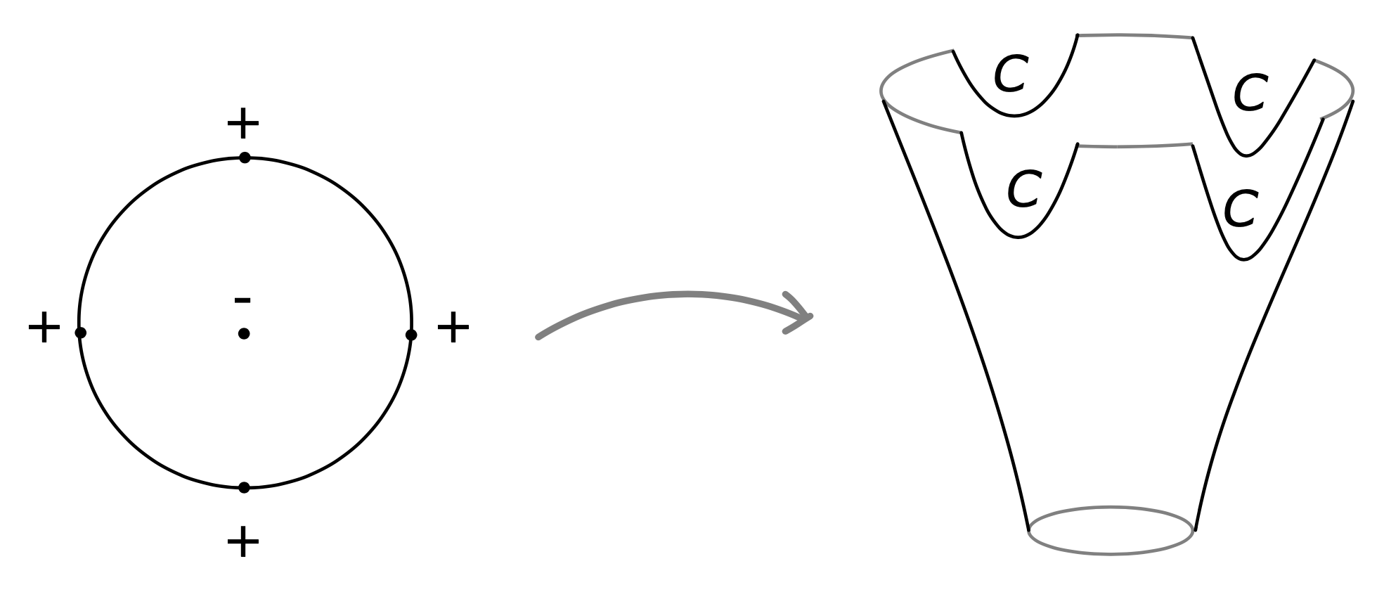
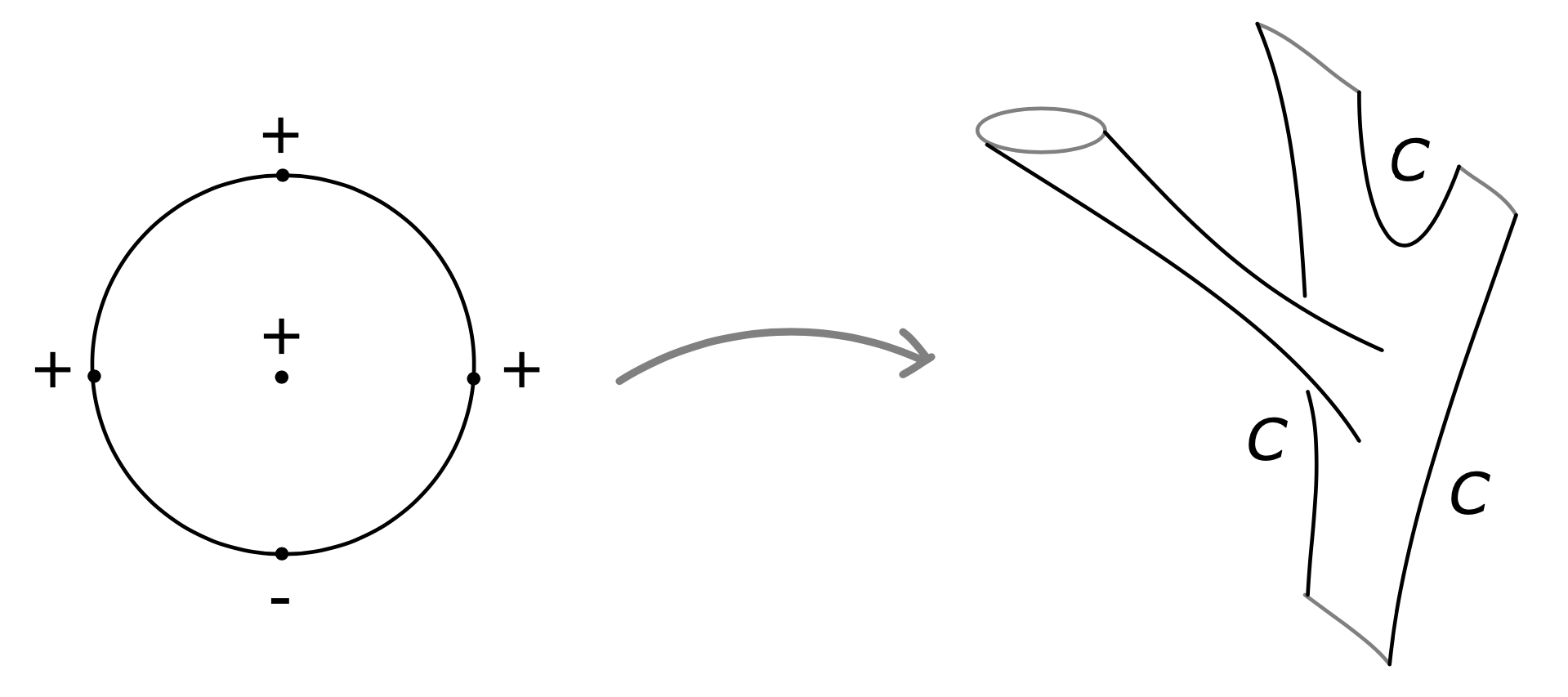
Consider now a Weinstein manifold \( X \). Using the equation \( L_{Z}\omega=\omega \), it is straightforward to check that the stable manifolds \( W^{\mathrm{s}} \) of the critical points are isotropic, that is, \( \omega \) vanishes along \( W^{\mathrm{s}} \). In particular, critical points have indices \( \le n \), and ordering the critical levels according to index then gives the following handle decomposition of \( X \): \[ \overline{X} = \overline{X}^n \supset \overline{X}^{n-1} \supset \dots \supset \overline{X}^{1} \supset \overline{X}^0, \quad \text{ where } \quad \overline{X}^{m} = \overline{X}^{m-1} \cup_{\Lambda^{m}} H^{m}, \quad m=1,\dots,n. \] Here \( \overline{X}^{0} \) is the \( 2n \)-ball and \( \overline{X}^{m} \) is obtained from \( \overline{X}^{m-1} \) by attaching \( m \)-handles \( H^{m}\approx \bigsqcup \overline{T^{\ast} D^{m}}\times B^{2(n-m)} \) along a collection of isotropic \( (m-1) \)-spheres \( \Lambda^{m} \) (the descending spheres of the isotropic stable manifolds) in the contact boundary \( Y^{m-1} \) of \( X^{m-1} \).
For \( m < n \) there is an \( h \)-principle for isotropic \( m \)-spheres in contact \( (2n-1) \)-manifolds, which means that the symplectic topology of \( X^{m} \) is uniquely determined by the homotopy class of the tangent map of \( \Lambda_{m} \). Consequently all the interesting symplectic topology of \( X=X^{n} \) is carried by the Legendrian isotopy class of the attaching spheres \( \Lambda=\Lambda^{n}\subset Y^{n-1}=\partial \overline{X}^{n-1} \). This observation can be taken as the starting point for the Legendrian surgery approach to symplectic topology invariants. It says that all symplectic invariants of \( X \) can be obtained from \( \Lambda \).
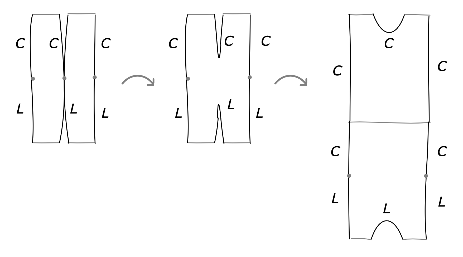
We will call the stable manifolds \( L \) of the index \( n \) critical points the core disks and the unstable manifolds \( C \) its cocore disks. The first Legendrian surgery result we will explain can then be stated as saying that the wrapped Floer cohomology \( CW^{\ast}(C) \) of \( C \) is quasiisomorphic to the Chekanov–Eliashberg dg-algebra \( CE^{\ast}(\Lambda) \) of \( \Lambda \).
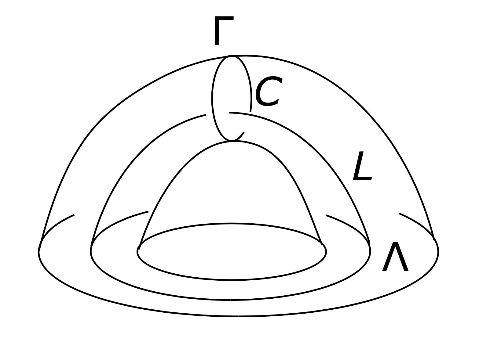
Below we will simplify notation and write \( \overline{X}=\overline{X}_{0}\cup_{\Lambda} H \), where \( \overline{X}_{0} \) is the subcritical part of \( X \), that is, the sublevel set of all handles of index \( < n \) and \( H \) is the union of critical \( n \)-handles, one copy of \( T^{\ast}D^{n} \) for each handle, attached along \( \Lambda\subset Y_{0}=\partial\overline{X}_{0} \). We will also simplify notation and write, for example, \( X=X_{0}\cup_{\Lambda} H \), etc., and not distinguish in notation between a Weinstein domain and the Weinstein manifold which is its completion. We use the notation \( Y=\partial_{\infty} X \) and \( Y_{0}=\partial_{\infty} X_{0} \) to denote ideal contact boundaries. Furthermore, we will write \( L \) and \( C \) for the stable and unstable manifolds of the index \( n \) critical points in \( H \), and call them the Lagrangian core and cocore disks, respectively. See Figure 1.
3. The basic surgery isomorphism
3.1. Reeb orbits and Reeb chords
Flow loops of \( R \) are called Reeb orbits. For generic contact form, Reeb orbits are isolated and transverse (linearized return map in general position). For our treatment of holomorphic curve theories we will use parameterized Reeb orbits. This means that we fix a point on each Reeb orbit and consider all its multiples parameterized, starting the parameterization at that point. If \( \Lambda\subset V \) is a Legendrian submanifold then Reeb chords of \( \Lambda \) are flow lines of \( R \) starting and ending on \( \Lambda \). Again, for generic data, Reeb chords are isolated and transverse (linearized flow from start point to endpoint in general position).
We next introduce the chain complexes underlying our main holomorphic curve theories. We start with the theory after handle attachment.
3.1.1. Generators of the wrapped Floer cohomology complex
Consider a Morse function \( f\colon C\to C \) with gradient equal to the Liouville vector field at infinity. Let \( C_{-} \) be a time \( -\epsilon \) shift along \( f \), viewed as a Hamiltonian in \( T^{\ast} C \). Then the wrapped Floer cohomology complex \( CW^{\ast}(C) \) of \( C \) is generated by Reeb chords starting on \( C \) and ending on \( C_{-} \) and intersection points in \( C\cap C_{-} \). Since the shift is small we see that generators correspond to Reeb chords of \( \Gamma \) and critical points of \( f \); see ([e8], Appendix B.1).
3.1.2. Generators of the Chekanov–Eliashberg dg-algebra
3.2. Handle attachment and Reeb dynamics
Proof. Outside the handle attachment region, the Reeb flows in \( Y_{0} \) and \( Y \) are naturally identified. We take the cocore as the fiber of \( T^{\ast} D \) at the center of \( D \). Inside the handle the Reeb flow is the lift of the geodesic flow. In particular, the Reeb flow takes fiber hemispheres of the attaching neighborhood to the boundary of the attaching region by a degree one map. A straightforward fixed point argument now establishes the 1-1 correspondence; see ([e4], Section 5) for details. □
3.3. Wrapped Floer cohomology
Proof. The square of the differential counts the ends of a 1-dimensional moduli space; see ([e8], Appendix B.1). □
In fact, the differential is the \( \mu_{1} \)-operation in an \( A_{\infty} \)-algebra structure on \( CW^{\ast}(C) \), where the operation \( \mu_{k} \) is defined by choosing \( k \) parallel copies of \( C \), where \( C_{-} \) is the first parallel copy which is the time \( -1 \) shift along the function \( \epsilon f_{1} \) for \( f_{1}=f \) and the \( k^\mathrm{ th} \) copy is the time \( -1 \) shift along the function \[ \left(\sum_{r=1}^{k} \epsilon^{k}\right) f_{1} + \left(\sum_{r=2}^{k} \epsilon^{3+r}\right)f_{2} + \dots + \epsilon^{k+1}f_{k}. \]
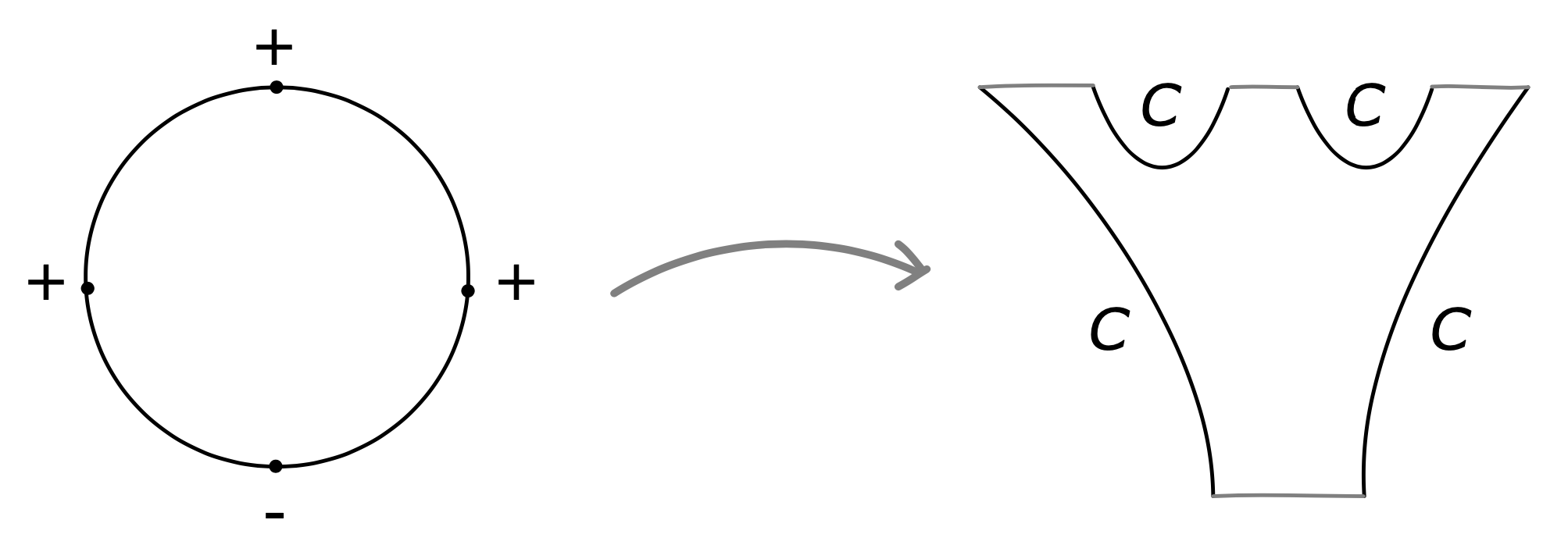
Then the \( \mu_{k} \)-operation counts disks with positive punctures connecting copies in increasing order and one negative output puncture; see Figure 2.
We then have the following result.
Proof.
Again the compositions count the ends of a 1-dimensional moduli space. The proof
requires that for sufficiently close parallel copies, moduli spaces with boundary
components on Lagrangians corresponding to any increasing numbering in the system of parallel copies
be canonically identified. This follows from the
form of the shifting functions and the fact that transversely
cut-out solutions persist under sufficiently small perturbation;
see
([e8], Appendix B.1).
□
3.4. The Chekanov–Eliashberg dg-algebra
We extend it to a dg-algebra differential by the Leibniz rule.
Proof. The square of the differential counts ends of a 1-dimensional moduli space; see, for example, [e8]. □
3.5. The chain map
We view \( CE^{\ast}(\Lambda) \) as an \( A_{\infty} \)-algebra generated by words of Reeb chords with differential \( \mu_{1}=\partial \), with \( \mu_{2} \) given by the concatenation product, and with all higher \( \mu_k \) equal to zero.
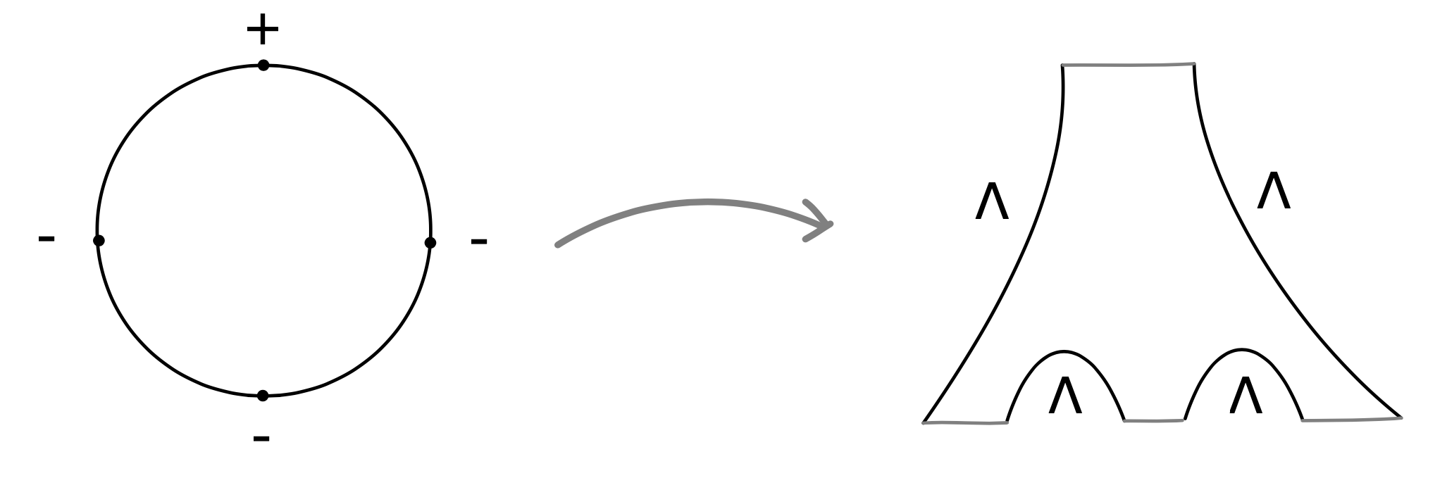
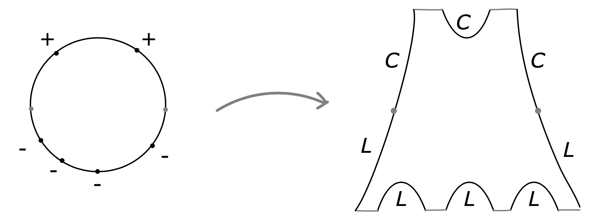
Proof. To see this we consider 1-dimensional moduli spaces of disks, as in the definition of \( \Phi_{k} \), and note that the boundary points of such a moduli do correspond to splittings at Reeb chords, which is precomposing \( \Phi_{k} \) with \( \mu_{j} \) in the positive end or postcomposing \( \Phi_{k} \) with \( \mu_{1} \) at the negative end, or splitting at one of the Lagrangian intersection points in \( C\cap L \), which corresponds to postcomposing \( \Phi_{j} \) with \( \mu_{2} \) in the negative end. The lemma follows; see ([e8], Appendix B.2) for more details. □
3.6. Chain isomorphism
Proof. The proof uses induction on action. For one-letter words an explicit construction gives one transversely cut-out strip which is unique by an action argument. Assume inductively that the count of curves in moduli space of disks connecting \( \overline{w} \) to \( w \) for all words of length \( \le m \) equals \( \pm 1 \). Then consider the moduli space of disks with two positive punctures at \( \overline{w}_{0} \) and \( \overline{w}_{1} \) and negative punctures at \( w_{0}w_{1} \). By action this moduli space has only two boundary breakings (see Figure 5): breaking at a point in \( C\cap L \), by induction we know that the count of such configurations equal \( \pm 1 \), and breaking into a disk with two positive and one negative puncture followed by an isomorphism disk, we conclude that both of these moduli spaces must also contain \( \pm 1 \) elements; see ([e4], Section 7). □
Using a straightforward action filtration argument (see ([e8], Appendix B.2)) we then get the main surgery isomorphism theorem:
4. Further results
4.1. Symplectic homology and linearized contact homology
Our complex for symplectic homology is thus Reeb orbits together with a Morse complex of the underlying geometric orbit and critical points of a Morse function on \( X \). The differential counts anchored holomorphic cylinders and spheres with Morse data at orbits; we call these decorated orbits. We denote the corresponding complex \( SC^{\ast}(X) \); see ([3], Section 3.3).
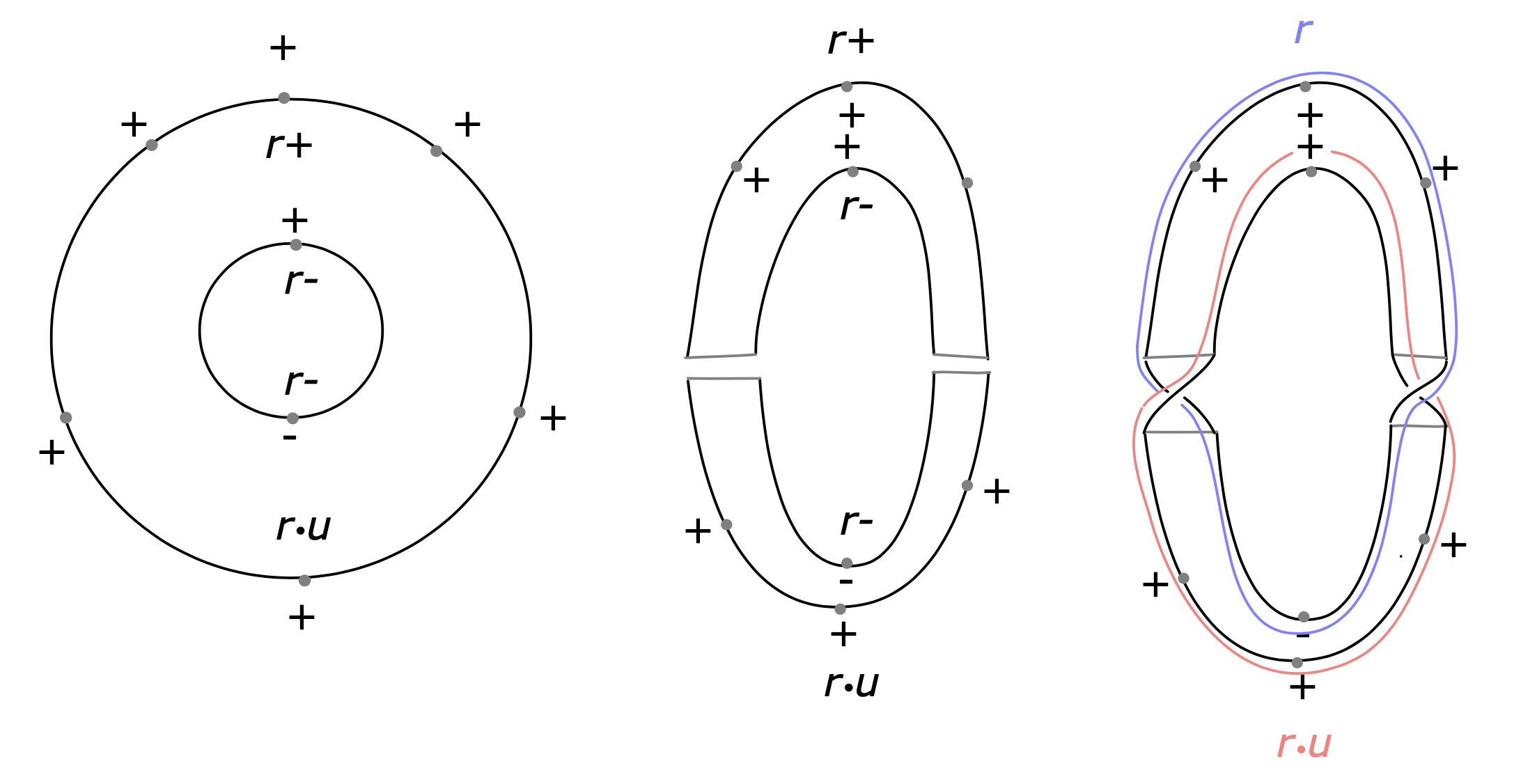
We next want to model this complex before surgery. The counterpart of Lemma 3.1 says that Reeb orbits after surgery are in natural 1-1 correspondence with Reeb orbits before surgery and cyclic words of Reeb chords of the attaching spheres; see ([e4], Section 5). In order to model this situation we use a two-copy \( L_0\cup L_{1} \) of the descending manifold. Here \( L_{0}\cap L_{1}=\{z\} \) is one point near the middle of the handle, and Reeb chords of the boundary of \( \Lambda_0\cup\Lambda_1 \) consist of two copies of Reeb chords of \( \Lambda \) and two additional Reeb chords \( x \) and \( y \) for each component of \( \Lambda \) corresponding to the maximum and a minimum of a Morse function making the Reeb shift generic.
We call a Reeb chord connecting \( \Lambda_0 \) to \( \Lambda_1 \) mixed and chords connecting \( \Lambda_{j} \) to itself pure. We then consider the two-copy Chekanov–Eliashberg dg-algebra complex which is generated by words of chords in which exactly one chord is mixed and others are pure. The differential counts holomorphic curves with mixed positive puncture, one mixed negative puncture, and any number of pure negative punctures. Rather than using this complex alone we use the (very small) Lagrangian Floer cohomology complex of \( L_0 \) and \( L_{1} \) with coefficients in the two-copy complex, where the differential also counts curves with one Lagrangian intersection point and negative end with one mixed puncture. In this case, this means simply add the generator \( z \) and observe that \( \partial z = y \). We denote this complex \( CF^{\ast}((L_{0},\Lambda_0),(L_{1},\Lambda_1)) \) and write simply \( \operatorname{H} CF^{\ast}(L,\Lambda) \) for the corresponding Hochschild complex that is obtained by identifying words up to cyclic permutation.
There is now a natural surgery cobordism map \[ \Phi^{SC}=\Phi_{\mathrm{o}}^{SC}\oplus\Phi_{\mathrm{w}}^{SC}\colon SC^{\ast}(X) \to SC^{\ast}(X_0)\oplus \operatorname{H} CF^{\ast}(L,\Lambda), \] where \( \Phi_{\mathrm{o}}^{SC} \) is the standard cobordism map counting cylinders between Morse decorated orbits, and where \( \Phi_{\mathrm{w}}^{SC} \) counts disks with positive puncture at a decorated orbit, mixed distinguished puncture at 1 and a puncture mapping to \( z \) at \( -1 \). We think of the right-hand side as a complex with differential \[ d = \left(\begin{matrix} d_{\mathrm{oo}} & d_{\mathrm{wo}}\\ d_{\mathrm{ow}} & d_{\mathrm{ww}} \end{matrix}\right), \] where \( d_{\mathrm{oo}} \) is the usual cylinder counting differential on \( SC^{\ast}(X_0) \), \( d_{\mathrm{wo}}=0 \), \( \,d_{\mathrm{ww}} \) is induced from the differential on \( \operatorname{H} CF^{\ast}(L,\Lambda) \), and where \( d_{\mathrm{ow}} \) counts disks with positive puncture at a Morse decorated orbit and distinguished negative puncture at mixed chord, similar to \( \Phi_{\mathrm{w}} \).
Proof. We adapt the Morse functions on the orbits corresponding to cyclic words so that these functions have a maximum and a minimum on each chord on the underlying orbit. It then follows that \( \Phi^{CW} \) takes an orbit with maximum on a chord \( c \) to the corresponding word of chords with the chord \( c \) mixed, and the orbit with a minimum on \( c \) to the corresponding word with \( c \) replaced by \( cx \), where \( c \) is the pure chord and \( x \) is the mixed chord at the minimum Reeb chord of the shift. The proof is then directly analogous to Theorem 3.7. □
This has the following consequence.
Proof. The complex \( SC^{\ast}(X_0) \) is contractible as the symplectic homology complex of a subcritical manifold. □
Combining Theorem 3.7 and Corollary 4.2 we learn that the Hochschild complex \( \operatorname{H} CW^{\ast}(C) \) of \( CW^{\ast}(C) \) is quasiisomorphic to the symplectic homology complex \( SC^{\ast}(X) \).
It is also possible to define the counterpart of \( SC^{\ast}(X) \) without Morse data on the orbits. The
corresponding complex is known as
cylindrical contact homology and is isomorphic to the \( S^{1} \)-equivariant
version of \( SC^{\ast}(X) \). The standard approach to defining this \( S^{1} \)-equivariant version is to define a
BV-operator that deforms the Hamiltonian perturbation by rotating the domain. This operation does not square to
zero and one has to add (infinitely many) correction terms. However, in the Morse–Bott description of
\( SC^{\ast}(X) \) the BV-operator \( \xi \) admits a simple description that does square to zero: if \( \gamma \) is a
Reeb orbit,
and \( \widehat{\gamma} \) and \( \check{\gamma} \)
denote \( \gamma \) decorated by a maximum and a
minimum, respectively, then \( \xi(\check{\gamma})=\widehat{\gamma} \) and \( \xi(\widehat{\gamma})=0 \). The
corresponding operation on cyclic words is \( \underline{x}w\mapsto \sum \underline{w} \), where the sum goes over
all ways of choosing mixed chord in \( w \). With this explicit form of the BV-operator it is straightforward to
obtain the cylindrical contact homology using a model for \( S^{1} \)-equivariant homology on \( \operatorname{H}
CF^{\ast}(L,\Lambda) \) together with the \( S^{1} \)-action given by the BV-operator \( \xi \) satisfying \( \xi^{2}=0 \).
4.2. Upside down surgery
By analogy with \( \Phi^{CW} \), we now have a chain map of infinity coalgebras \[ \Phi_{CW}\colon \operatorname{B} CW^{\ast}(C)\to LCE^{\ast}(\Lambda). \] Here the left-hand side is the bar complex of \( CW^{\ast}(C) \), that is, \( \operatorname{B} CW^{\ast}(C) \) is generated by words of Reeb chords of \( \Gamma \) and critical points in \( C \) with differential induced by the \( \mu_{k} \)-operations. This bar complex \( \operatorname{B} CW^{\ast}(C) \) is naturally a (infinity) coalgebra with differential \( c_1 \), coproduct \( c_2 \) corresponding to splitting words in two all possible ways and all higher \( c_{k} \) equal to zero. The right-hand side is the linearized Chekanov–Eliashberg dg-algebra (here we assume that \( CE^{\ast}(\Lambda) \) has an augmentation) where the operations \( c_{k} \) correspond to the part of the (augmented) differential with \( k \) negative punctures. In direct analogy with Theorem 3.7 we have the following.
We consider also the cyclic version of this map. We start from the Hochschild complex \( \operatorname{H} CW^{\ast}(C) \) of \( CW^{\ast}(C) \) generated by cyclic words of Reeb chords, one of which is distinguished. In analogy with the core disk, we think of this as a two-copy complex where the distinguished puncture is mixed and where we also have the intersection point \( z=C_{0}\cap C_1 \) as a generator with \( \partial z=x \), where is the minimum of the Reeb shift at infinity and where the maximum \( y \) of the Reeb shift plays a role analogous to \( x \) for the two copy of \( L \). We then add to \( \operatorname{H} CW^{\ast}(C) \) the complex \( SC^{\ast}(X) \). The differential counts, except for the usual curves also disks with several positive punctures and a negative puncture at the center, the location of the distinguished positive puncture at a fixed boundary location determined by the marker at orbit in the center and an antipodal puncture mapping to \( z \). We denote this complex \[ \operatorname{H} CW^{\ast}(C)\oplus SC^{\ast}(X) \] and in analogy with Theorem 4.1 we have a natural chain map \[ \Psi\colon \operatorname{H} CW^{\ast}(C)\oplus SC^{\ast}(X) \to SC^{\ast}(X_{0}) \] which is a chain isomorphism. The connecting homomorphism in the long exact sequence associated to the short exact sequence \[ 0 \to SC^{\ast}(X) \to \operatorname{H} CW^{\ast}(C)\oplus SC^{\ast}(X) \to \operatorname{H} CW^{\ast}(C) \to 0 \] is called the open-closed map; see [e1], [e2]. We will denote it \[ \mathcal{OC}\colon \operatorname{H} CW^{\ast}(C)\to SC^{\ast}(X). \] See Figure 6.
Since \( SC^{\ast}(X_{0}) \) is contractible we find:
4.3. The closed-open map and isomorphisms of Hochschild homology and cohomology
The Hochschild chain complex \( \operatorname{H} CW^{\ast}(C) \) above can be thought of as generated by words of negative punctures at Reeb chords along the boundary of a formal disk (one of which is distinguished, we take it to be mixed). The Hochschild differential then attaches holomorphic disks with several positive and one negative puncture to such words in all possible ways (the negative and one of the positive punctures mixed). Similarly, we consider the Hochschild cochain complex \( \operatorname{H}^{\prime} CW^{\ast}(C) \) generated by chords along the boundary of a formal disk, all positive except one which is negative (as in the differential the negative and one positive puncture mixed). The differential on \( \operatorname{H}^{\prime} CW^{\ast}(C) \) is obtained by attaching the disks corresponding to the differential on \( \operatorname{H} CW^{\ast}(C) \) with one negative and several positive punctures in all possible ways, from above and below.
The complex \( \operatorname{H}^{\prime} CW^{\ast}(C) \) has a natural product which acts by gluing negative and positive punctures of one to the other. This product has a natural unit \( e \) which is the sum of words of two-punctured disks with the same chord at the positive and negative puncture. Furthermore, there is a curve-counting map, the closed-open map \[ \mathcal{CO}\colon SC^{\ast}(X)\to \operatorname{H}^{\prime} CW^{\ast}(C), \] which counts disks with a positive puncture with a marker at the center mapping to an orbit with Morse decoration, one mixed negative boundary puncture at a fixed position, and any number of positive boundary punctures with the mixed chord at the point opposite the fixed position; see Figure 7.
Proof. The symplectic cohomology product followed by the isomorphism gives a disk with two positive punctures. Looking at possible splittings we find the product on the Hochschild cochains up to exact terms. □
Consider now the complex \( \operatorname{H} CW^{\ast}(C) \). This is naturally a \( \operatorname{H}^{\prime}CW^{\ast}(C) \)-module: if \( a\in \operatorname{H} CW^{\ast}(C) \) is a cyclic word and \( r\in\operatorname{H}^{\prime} CW^{\ast}(C) \), then \( r\cdot a \) is the sum of cyclic words obtained by attaching the positive punctures of \( r \) to consecutive (negative) punctures of \( a \). Precomposing the product by the map \( \mathcal{CO} \) we find that \( \operatorname{H} CW^{\ast}(C) \) is also an \( SC^{\ast}(X) \)-module. The symplectic homology complex has the pairs-of-pants product and is hence an \( SC^{\ast}(X) \)-module itself. We have the following.
Proof. The boundary of the 1-dimensional (reduced) moduli spaces of curves with positive chord punctures at the boundary, one negative and one positive interior puncture on the distinguished ray from the center to the distinguished puncture, correspond exactly to first multiplying and then applying the isomorphism or first applying the isomorphism and then multiplying. □
Together with a degeneration of moduli spaces argument, this leads to the following result.
Proof.
We use two parallel fibers \( C_0 \) and \( C_1 \) as source of the map \( \mathcal{OC} \) and target of the map \( \mathcal{CO} \), respectively. We will take them to
lie close together. Note that for the Legendrians at infinity of the parallel fibers, the shift from \( \partial_{\infty}C_0 \) to \( \partial_{\infty} C_{1} \) is induced by a Morse function on the sphere that is the restriction of a linear function that is negative at the south pole, vanishes on the equator, and positive at the north pole. Note then that Reeb chords \( C_0\to C_1 \) and \( C_1\to C_0 \) correspond to Reeb chords \( C\to C \) and short Reeb chords near \( C_0 \), and that therefore, there is a natural 1-1 correspondence between Reeb chords \( C_0\to C_{1} \) and Reeb chords \( C_1\to C_0 \).
We remark that when we discuss moduli spaces of holomorphic curves for the Lagrangians \( C_0 \) and \( C_{1} \) below, we need to use systems of parallel copies as described above. We use separate systems for \( C_{0} \) and \( C_{1} \) (see ([e8], Appendix B)), but will leave these systems implicit in the notation.
Let 1 denote the unit in \( SC^{\ast}(X) \). In the complex \( SC^\ast(X) \), 1 is represented by the minimum of the Morse function on \( X \). Since \( \mathcal{CO} \) is an isomorphism, we find \( u\in \operatorname{H} CF^{\ast}(C) \) such that \( \mathcal{OC}(u)=1 \). Take \( s\in SC^{\ast}(X) \). Then, since \( \mathcal{OC} \) is a map of \( SC^{\ast}(X) \)-modules with the module structure on \( \operatorname{H} CF^{\ast}(C) \) induced by \( \mathcal{CO} \) followed by the natural action of \( \operatorname{H}^{\prime} CF^{\ast}(C) \) on \( \operatorname{H} CF^{\ast}(C) \), we find \[ \mathcal{OC} ( \mathcal{CO} (s) \cdot u )= s\cdot \mathcal{OC}(u)=s\cdot 1=s. \] It follows that \( \mathcal{CO} \) is injective.
To show that \( \mathcal{CO} \) is surjective, note that \( \mathcal{CO}(1) \) counts curves with a positive puncture at the minimum on \( X \). The only such curves correspond to flow lines starting at the minimum and ending at a fixed point (the midpoint, say) of any Reeb chords. It follows that \[ \mathcal{CO}(1) = e =\sum_{\text{Reeb chords } c} c_{\mathrm{pos}}\otimes c_{\mathrm{neg}}. \]
Consider the moduli spaces \( \mathcal{M}(u;e) \) involved in the equation \[ \mathcal{CO}\circ\mathcal{OC}(u) = e. \] The elements in these moduli spaces are infinite-length cylinders with positive punctures corresponding to \( u \) at one boundary component and one positive and one negative puncture along the other boundary component corresponding to any chord in \( e \). Gluing at the middle orbit we gain one dimension since the marker in the middle disappears. This means that the resulting moduli space has dimension two.
Consider a cycle \( r\in \operatorname{H}^{\prime} CF^{\ast}(C) \) and a nontrivial contribution to \( r\cdot u \). We use this contribution to degenerate the moduli spaces in \( \mathcal{M}(u;e) \). We degenerate the annulus into two disks \( D_{\mathrm{up}} \) with positive punctures according to the positive punctures in \( r \) and the positive puncture in the \( e \)-term corresponding to the negative puncture of \( r \), and two negative punctures, and a disk \( D_{\mathrm{dn}} \) in the lower part with positive punctures at the chords in \( r\cdot u \) that are not the negative chord of \( r \). Under this deformation the moduli space undergoes additional splittings that will only affect the result up to exact terms, using the assumptions that \( r \) and \( u \) are cycles.
We next glue \( D_{\mathrm{up}} \) and \( D_{\mathrm{dn}} \) via a cobordism corresponding to an isotopy that interchanges \( \partial C_0 \) and \( \partial C_1 \). The Lagrangian cobordism \( T\subset \mathbb{R}\times\partial X \) corresponds to the Legendrian isotopy in \( \partial X \) that rotates \( \partial C_0 \) to \( \partial C_1 \), and then takes the shifting function to its negative. It is easy to see that if \( C_0 \) and \( C_1 \) are sufficiently close and the rotation is sufficiently slow, all rigid holomorphic curves in the cobordism corresponds to (reparameterized) trivial Reeb chord strips of \( c \) and strips (corresponding to Morse flow lines) that interchanges the small Reeb chords that follows the rotation. Let \( \mathcal{M}(T) \) denote the moduli space of rigid holomorphic curves with boundary on \( T \).
Noting that the curves in \( \mathcal{M}(T) \) are strips that exactly give the natural 1-1 correspondence between Reeb chords \( C_0\to C_1 \) and \( C_1\to C_0 \), we find that the result of gluing \( D_{\mathrm{dn}} \) via \( \mathcal{M}(T) \) to \( D_{\mathrm{up}} \) are new annuli of dimension 2 that have positive punctures according to \( r\cdot u \) along one boundary component and positive and one negative puncture according to \( r \). Then, deforming the Lagrangians to the standard \( C_0\cup C_1 \) and following the domains until it splits at a Reeb orbit, we find that \[ \mathcal{CO}(\mathcal{OC}(r\cdot u))=r, \] up to exact terms; see Figure 8. It follows in particular that \( \mathcal{CO} \) is surjective. The theorem follows. □
4.4. The symplectic homology product and Calabi–Yau structures
In order to compute the product we consider the composition \[ \Phi^{SC}\circ \mu\colon SC^{\ast}(X)\otimes SC^{\ast}(X)\to \operatorname{H} CE^{\ast}(\Lambda). \] The curves contributing to this composition are disks with two positive punctures near the origin and negative boundary punctures and one extra puncture opposite the distinguished mixed puncture mapping to \( z \). As in the proof of Theorem 4.8, at the gluing we gain one dimension from a disappearing conformal constraint. We use it to control the conformal structure of the domain. Studying splittings we find the following; see [2].
4.5. Partial wrapping and coefficients in chains of the based loop space
This translation shows that any construction in exact Floer theory admits a surgery description and gives, for example, a rather direct and geometric proof of the cut-and-paste methods of [e9]; see ([e6], Theorem 1.3) and ([e7], Theorem 1.1). Here we will illustrate the idea by giving the definition of the surgery description of partially wrapped Floer cohomology and a sample result that can be proved with this technology.
Consider Weinstein domains \( W \) of dimension \( 2n \) and \( V \) of dimension \( 2n-2 \). We fix a Lagrangian skeleton \( L \) with a fixed handle structure for \( V \) and think of \( V \) as a cotangent bundle of \( L \). We take a Legendrian embedding of \( L \) into \( \partial W \) to be a contact embedding of a neighborhood \( V\times (-\epsilon,\epsilon) \) of the zero section in the contactization of \( V \). Given such an embedding, consider \( W \) with the fixed embedding of \( V\times (-\epsilon,\epsilon) \) in \( \partial W \) and also the negative half \( [0,-\infty)\times\mathbb{R}\times V \) of the symplectization of \( \mathbb{R}\times V \) with \( V\times (-\epsilon,\epsilon)\times V \) embedded in \( \{0\}\times \mathbb{R}\times V \). We attach a \( V \)-handle, \( T^{\ast} I\times V \), to the union. Note that the handles of \( V \) give attaching spheres for \( X \). We define the Chekanov–Eliashberg dg-algebra of \( L \) to be the Chekanov–Eliashberg dg-algebra of the Legendrian attaching spheres of \( X \). Note that it is generated by Reeb chords of \( L \) together with Reeb chords of the Legendrian attaching spheres in \( V \) in the middle of the handle.
In case \( L \) is smooth, observe that the internal Reeb chords of \( L \) give a dg-algebra quasiisomorphic to the chains on the based loop space of \( L \). Using this observation one can show that the dg-algebra of \( L \) is then isomorphic to the dg-algebra with loop space coefficients; see ([e6], Theorem 1.2).
We give one illustration of how this construction can be used. Consider a smooth manifold \( M \) and fix a Morse function \( f\colon M\to\mathbb{R} \) with one maximum and one minimum. It is well known that the wrapped Floer cohomology of the cotangent fiber in \( T^{\ast} M \) is quasiisomorphic to chains on the based loop space of \( M \), \[ CW^{\ast}(T_{m}M)\approx C_{\ast}(\Omega M). \] For the purposes of this discussion, we think of this result as not cutting \( M \) at all, or to comply with what comes next, as cutting \( M \) below the minimum of the Morse function. We can also cut \( M \) just below the maximum. If \( M_{\le a} \) is the sublevel set then the cotangent bundle \( T^{\ast}M_{\le a} \), with corners rounded, is a subcritical Weinstein domain with the level sphere \( \Lambda_{a}=\partial M_{\le a} \) as a Legendrian submanifold. By the surgery isomorphism, Theorem 3.7, \( \,CE^{\ast}(\Lambda_{a}) \) is also isomorphic to \( CW^{\ast}(T_{m} M) \). It turns out the same holds true if we cut at any regular level \( b \). More precisely, we get a subcritical Weinstein domain \( T^{\ast}M_{\le b} \) with a Legendrian level surface \( \Lambda_{b}=f^{-1}(b) \). Consider now the Chekanov–Eliashberg dg-algebra of \( \Lambda_{b} \) with coefficients in chains of the based loop space of the superlevel set \( M_{\ge b} \), \[ CE^{\ast}(\Lambda_{b};C_{\ast}(\Omega(M_{\ge b}))). \] Then, in fact, \begin{equation} CE^{\ast}(\Lambda_{b};C_{\ast}(\Omega(M_{\ge b}))) \approx CW^{\ast}(T_{m}^{\ast}M), \tag{4.1} \end{equation} for every regular value \( b \). The isomorphisms in Equation (4.1) illustrate the fact that in the exact case, Floer cohomology can be expressed either in terms of topology or Reeb dynamics, and further that it is possible to interpolate between these extreme cases by having a part in topology and another in Reeb dynamics.
The isomorphisms in this example are straightforward to derive, working in Legendrian surgery presentations. We describe them here as an illustration of the great generality and flexibility of Eliashberg’s original surgery approach to holomorphic curve theories in Weinstein domains. It can handle very general objects, and provides, for example, Chekanov–Eliashberg dg-algebra or Floer cohomology for Legendrians with boundary with corners with coefficients in chains on the based loop space, in terms of the usual dg-algebras of Legendrian attaching spheres in suitable Weinstein manifolds. Such singular Lagrangians and Legendrians are very useful for instance as centers of mirror symmetry charts; see [e5] for a simple example.
Tobias Ekholm is a professor of mathematics at Uppsala University and Director of Institut Mittag-Leffler.
