by Lenhard L. Ng and Joshua M. Sabloff
In this brief celebration, we honor Yasha Eliashberg’s contributions to the foundations of transverse and (especially) Legendrian knot theory. We assume familiarity with basic notions of Legendrian and transverse knots in the standard contact \( (\mathbb{R}^3, \ker(dz - y\, dx)) \), including the front projection to the \( xz \)-plane and the Lagrangian projection to the \( xy \)-plane. We also assume knowledge of the classical invariants: the Thurston–Bennequin invariant \( \operatorname{tb} \) (which measures the twisting of the contact planes around a Legendrian knot), the rotation number \( \operatorname{rot} \) (which measures the twisting of a Legendrian knot in the contact planes), and the self-linking number \( \operatorname{sl} \) (which measures the contact framing of a transverse knot). See Etnyre’s survey [e13] or Geiges’ text [e17] for thorough introductions.
Our goal is to pay tribute to Eliashberg’s work rather than exhaustively survey the field — the impossibility of compactly surveying the entire field is, itself, a testament to his influence — and hence our citations will be sparse and will focus on a combination of older foundational work and more recent surveys. We note for the experts that we will occasionally adopt some nontraditional conventions in order to simplify the exposition for nonexperts.
The present authors gratefully acknowledge that they are among the many mathematicians whose research has been shaped by Eliashberg’s ideas in Legendrian and transverse knot theory.
1. Origins of Legendrian and transverse knot theory
Legendrian and transverse knots have long played a central role in contact topology. For example, Martinet’s proof in the early 1970s that every closed, orientable 3-manifold carries a contact structure relies on surgery along transverse links [e2]. Further, Lutz proved that every co-oriented 2-plane field on a closed, orientable 3-manifold is homotopic to a contact structure using modifications of contact structures in neighborhoods of transverse links [e1].
A decade after Lutz’s and Martinet’s work,
Bennequin
[e3]
demonstrated that the
theory of Legendrian and transverse knots in the standard contact \( \mathbb{R}^3 \) is interesting
in itself. In particular, Bennequin proved what is now called the
Bennequin
Inequality:
for any Seifert surface \( F \) of a transverse knot \( T \), we have
\[
\operatorname{sl}(T) \leq -\chi(F).
\]
It follows that the Thurston–Bennequin number of a Legendrian knot satisfies a similar
bound. This bound can be used to demonstrate the existence of exotic contact structures
on \( \mathbb{R}^3 \).
In the early 1990s, Eliashberg expanded on both of these early threads, pushing the field in new directions. First, Eliashberg’s paper [3], along with Weinstein’s work [e4], demonstrated the importance of surgery on Legendrian, rather than transverse, knots; see also [e5]. Legendrian surgery arises from attaching a symplectic handle, thus connecting the topology of contact manifolds to that of the symplectic manifolds that they bound. Second, in [4], Eliashberg generalized Bennequin’s Inequality to any “tight” contact 3-manifold, thereby establishing the importance of Legendrian and transverse knots in understanding rigidity phenomena in contact topology. In particular, he proved that if \( T \) is a null-homologous transverse knot in a tight contact 3-manifold \( M \), then for any relative class \( \mu \in H_2(M,K) \) and surface \( F \) representing \( \mu \), we have \[ \operatorname{sl}(T; \mu) \leq -\chi (F). \] The technique underlying the proof was the manipulation of the characteristic foliation on \( F \), which is a 1-dimensional foliation on \( F \) induced by the contact structure. It was already known, in large part because of Eliashberg’s work with Thurston [7], that foliations provided a powerful way to analyze contact structures on 3-manifolds. Eliashberg used the tightness hypothesis and the elimination of singularities to simplify the characteristic foliation on the surface \( F \) until the generalized Bennequin Inequality was revealed.
Both the centrality of the tight vs. overtwisted dichotomy in contact topology and the importance of Legendrian surgery will be discussed elsewhere in this volume.
The paper [4] also introduced the geography and botany questions that, to this day, frame the study of Legendrian and transverse knots. Letting \( \mathcal{E} \) be the set of isotopy classes of smooth knots, \( \mathcal{T} \) be the set of transverse isotopy classes of transverse knots, and \( \mathcal{L} \) be the set of Legendrian isotopy classes of Legendrian knots, Eliashberg introduced the functions \begin{align*} \tau: \mathcal{T} &\to \mathcal{E} \times \mathbb{Z}, & \lambda: \mathcal{L} &\to \mathcal{E} \times \mathbb{Z} \times \mathbb{Z}, \\ T &\mapsto (K_T, \operatorname{sl}(T)), & \Lambda & \mapsto (K_\Lambda, \operatorname{tb}(\Lambda), \operatorname{rot}(\Lambda)), \end{align*} where \( K_* \) denotes the underlying smooth knot type. He then asked:
- Geography: What are the images of \( \tau \) and \( \lambda \)? That is, which classical invariants can be realized by transverse and Legendrian knots? Given that the Bennequin Inequality yields upper bounds on the \( \operatorname{sl} \) and \( \operatorname{tb} \) for a given smooth knot type, Eliashberg proposed that an important first step would be to understand the maximal \( \operatorname{sl} \) and \( \operatorname{tb} \) among transverse and Legendrian realizations of a given smooth knot type; see [e16] for a summary of progress on this aspect of the geography question.
- Botany: To what extent, if at all, do the functions \( \tau \) and \( \lambda \) fail to be injective? That is, are there examples of distinct Legendrian or transverse knots with the same classical invariants?
From this point on, we will concentrate our discussion on Eliashberg’s influence of Legendrian knot theory.
2. Classification of Legendrian knots
Having established the guiding geography and botany questions, Eliashberg also provided the first classification result for Legendrian and transverse knots. In [4], Eliashberg established a complete classification of unknotted transverse knots in standard contact \( \mathbb{R}^3 \), and stated a parallel conjectural classification of Legendrian unknots. This Legendrian classification was completed by Eliashberg and Fraser in an influential pair of papers [6], [9].
The first sentence in Theorem 2.1 answers the botany question for Legendrian unknots, and the second one answers the geography question. Note that for the geography question, the first condition on the pair \( (\operatorname{rot},\operatorname{tb}) \) in Theorem 2.1 follows from Bennequin’s Inequality as described in Section 1, while the second condition follows from a straightforward computation in algebraic topology.
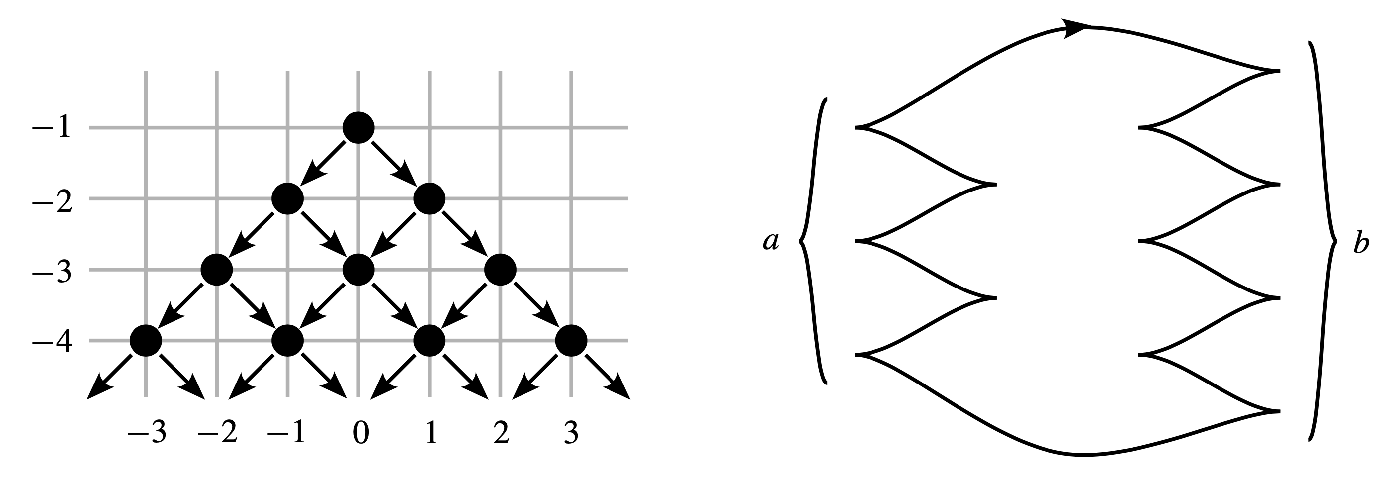
Theorem 2.1 implies that there is a one-to-one correspondence between Legendrian unknots, up to Legendrian isotopy, and pairs of integers \( (\operatorname{rot},\operatorname{tb}) \) satisfying the stated conditions. Thus we may depict the collection of Legendrian unknots by plotting the possible values of \( (\operatorname{rot},\operatorname{tb}) \) in \( \mathbb{Z}^2 \). This is shown in the left-hand diagram in Figure 1. Representatives of each of these unknots are shown in the right-hand diagram in Figure 1.
The arrows in the plot of \( (\operatorname{rot},\operatorname{tb}) \) in Figure 1 represent the geometric operations \( S_\pm \) called positive and negative stabilization, which start with a Legendrian knot and produce another one by inserting a zigzag along the front. The Thurston–Bennequin and rotation numbers change under stabilization as follows: \[ (\operatorname{rot}(S_\pm(\Lambda)),\operatorname{tb}(S_\pm(\Lambda)) = (\operatorname{rot}(\Lambda)\pm 1,\operatorname{tb}(\Lambda)-1). \] Each of the Legendrian unknots shown in Figure 1 is the result of applying a sequence of stabilizations to the “flying-saucer” unknot with \( (a,b)=(1,1) \) and \( (\operatorname{rot},\operatorname{tb}) = (0,-1) \); in the \( (\operatorname{rot},\operatorname{tb}) \)-plane, this unknot forms the peak of the mountain of Legendrian unknots.
More generally, the plot of possible values of \( (\operatorname{rot},\operatorname{tb}) \) for Legendrian representatives of some topological knot type is commonly called the Legendrian mountain range for the knot, with peaks corresponding to specific Legendrian knots, and mountains below those peaks coming from applying stabilizations. The resulting Legendrian mountain range is a visual representation of the geography for the smooth knot type.
The heart of Theorem 2.1 is the first sentence, solving the botany question for Legendrian unknots. To prove this, Eliashberg and Fraser applied the theory of characteristic foliations. Following in the footsteps of earlier work of Eliashberg [4], described above, they studied the characteristic foliation on a disk in \( \mathbb{R}^3 \) bounded by a Legendrian unknot. They argued that one could deform the disk in such a way that the characteristic foliation took a standard form, at which point the Legendrian unknot also assumed a standard form.
In the decades since the pioneering work of Eliashberg and Fraser, the strategy of studying Legendrian knots through characteristic foliations has achieved central importance in the theory of Legendrian knots. It arguably underlies Giroux’s hugely important theory of convex surfaces, which in turn has produced more classification results for Legendrian knots of knot types besides the unknot. There are now too many classification results to properly discuss here, but we illustrate the nature of these types of results through two examples: Legendrian torus knots, which were classified by Etnyre and Honda [e7], and Legendrian twist knots, which were classified in [e7], [e19].
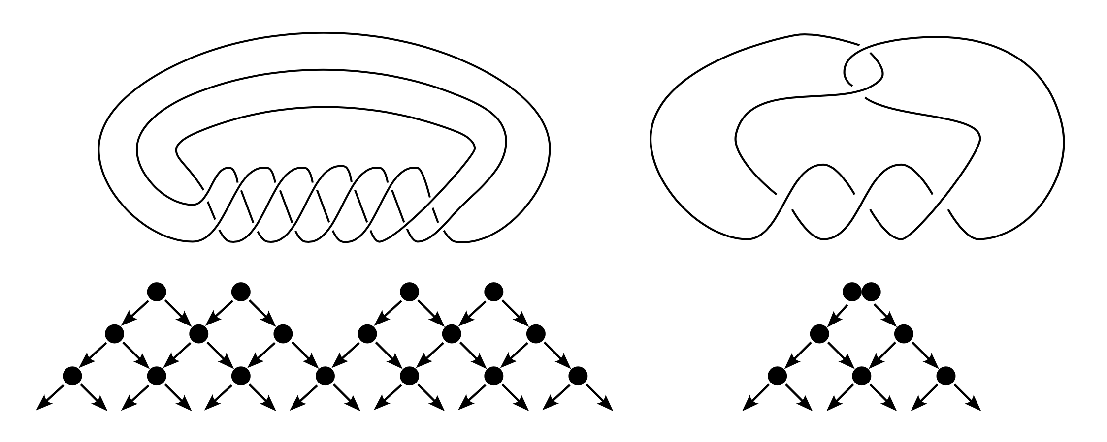
Using techniques inspired by Eliashberg and Fraser, Etnyre and Honda showed that just as for the unknot, torus knots are Legendrian simple: two Legendrian representatives of one of these knot types are Legendrian isotopic if and only if they share the same \( (\operatorname{rot},\operatorname{tb}) \). This answers the botany question for these knots. Etnyre and Honda completed the classification of Legendrian torus knots by determining the Legendrian mountain range for each torus knot. One example, for the \( (-7,3) \) torus knot, is illustrated in Figure 2.
Legendrian twist knots were similarly classified in [e19], again using techniques derived from Eliashberg–Fraser. Here there is a new wrinkle related to the botany question: some twist knots are not Legendrian simple, meaning that there are distinct Legendrian representatives with the same \( (\operatorname{rot},\operatorname{tb}) \). One such knot is \( m(5_2) \), the mirror of the \( 5_2 \) knot, whose Legendrian mountain range is shown in Figure 2: this has two distinct representatives with \( (\operatorname{rot},\operatorname{tb})=(0,1) \), as we will discuss in the following sections.
Many more classification results are now known for various knots (and links; see, e.g., [e15]) in both standard contact \( \mathbb{R}^3 \) and other contact 3-manifolds. In the latter category, Eliashberg and Fraser’s work in [9], and Dymara’s independent and more detailed work in [e8], classified unknots in overtwisted contact structures on \( \mathbb{R}^3 \) in addition to the standard tight contact structure. They discovered that Eliashberg’s tight-versus-overtwisted dichotomy leads to a dichotomy of Legendrian knots in overtwisted contact structures: loose versus nonloose, with loose knots encompassing those where the contact structure on the complement of the knot is still overtwisted. The classification problem is significantly easier for loose unknots than for nonloose ones. The concept of loose/nonloose knots now plays a central role in the study of Legendrian knots in general overtwisted contact 3-manifolds.
In studying the botany problem for Legendrian knots, Eliashberg’s characteristic foliation techniques are useful in circumstances where one needs to prove that two Legendrian knots must be Legendrian isotopic. In other circumstances, as for the \( m(5_2) \) knot, one wants to prove that two Legendrian knots are not Legendrian isotopic. For this, it is important to have strong invariants of Legendrian knots under Legendrian isotopy. Eliashberg was also a pioneer in this area, as we shall discuss in the remainder of this article.
3. Legendrian contact homology
One of the most significant developments in the past 30 years in Legendrian knot theory was the
introduction of the invariant now commonly called Legendrian contact homology (LCH for short). Eliashberg
and his collaborators laid out a general framework for Legendrian contact homology in the late 1990s, and
it has subsequently created an explosion of research in contact topology. There are now already many dozens
of papers whose reviews on
\href{https://mathscinet.ams.org/mathscinet/publications-search?query=any
[5],
and in more detail (though still just in outline form) by Eliashberg,
Givental,
and
Hofer
in
[8].
Despite the importance that it would eventually assume in contact topology, Legendrian contact
homology was mainly treated in these original papers as an offshoot of other things: a relative
version of contact homology for closed contact manifolds, which itself was only the first floor of
the multistory building of symplectic field theory (SFT). Contact homology and SFT are discussed in detail in other articles in this volume; here we will concentrate specifically on Legendrian contact homology.
Roughly speaking, LCH is the homology of a differential graded algebra \( (\mathcal{A},\partial) \) that incorporates a Floer-theoretic count of (pseudo)holomorphic curves associated to a Legendrian submanifold. More specifically, let \( (V,\alpha) \) be a contact manifold equipped with a contact 1-form \( \alpha\in\Omega^1(V) \), and let \( \Lambda \subset V \) be a Legendrian submanifold. The symplectization of \( (V,\alpha) \) is the symplectic manifold \( (V\times\mathbb{R},d(e^t\alpha)) \) where \( t \) is the coordinate on \( \mathbb{R} \); the cylinder \( \Lambda\times\mathbb{R} \) is a Lagrangian submanifold of \( V\times\mathbb{R} \). Assume for simplicity that \( V \) has no closed Reeb orbits — this happens, for instance, when \( (V, \alpha) \) is the standard contact \( \mathbb{R}^3 \) — though Eliashberg, Givental, and Hofer [8] propose a more elaborate story when \( V \) does have closed Reeb orbits.
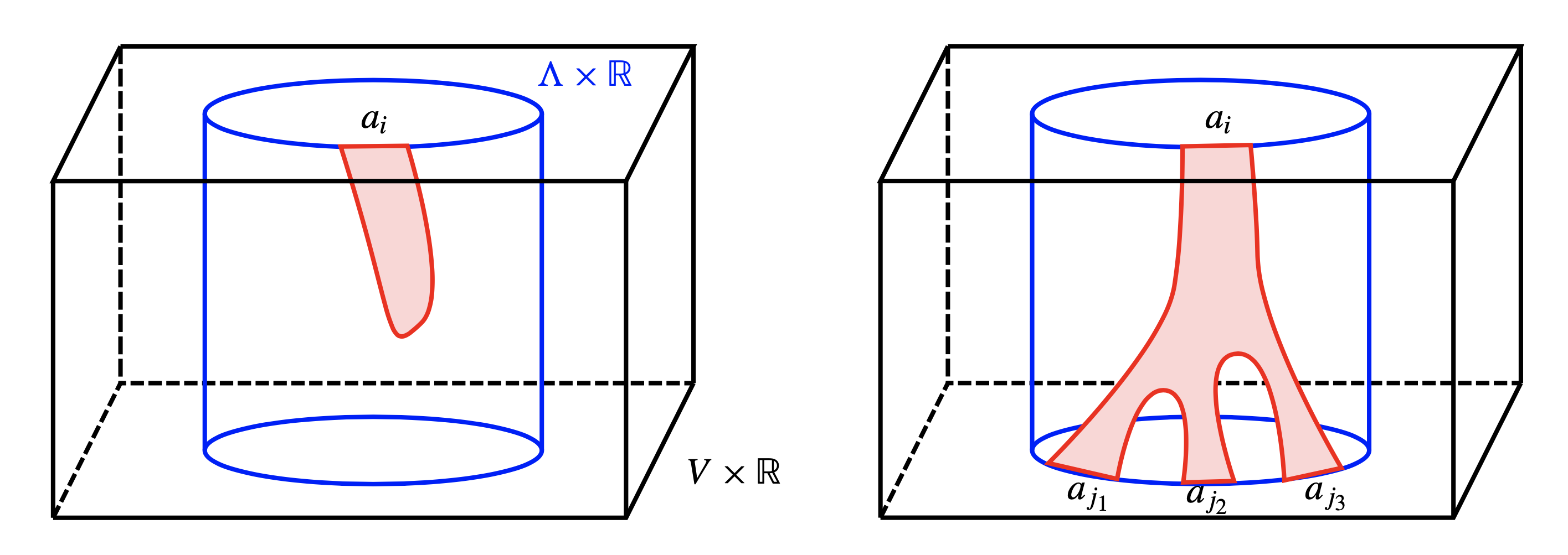
The algebra \( \mathcal{A} \) associated to the Legendrian \( \Lambda \) is a (noncommutative, unital) tensor algebra freely generated by the Reeb chords of \( \Lambda \). The differential \( \partial \) of a generator \( a_i \) is a sum of terms of the form \( a_{j_1}\cdots a_{j_k} \) over moduli spaces \[ \mathcal{M}(a_i;a_{j_1},\dots,a_{j_k}) \] of rigid holomorphic disks in \( V\times\mathbb{R} \) with boundary on the Lagrangian cylinder \( \Lambda\times\mathbb{R} \), a single “positive end” asymptotic to the Reeb chord \( a_i \) at \( +\infty \) in the \( \mathbb{R} \) direction, and any number of “negative ends” asymptotic to Reeb chords \( a_{j_1},\dots,a_{j_k} \) at \( -\infty \). (If we replace “holomorphic disks” by “holomorphic spheres” without boundary, and “Reeb chords” by “Reeb orbits”, then a similar sum enters into the definition of usual contact homology.) See Figure 3 for an illustration.
After constructing the DGA \( (\mathcal{A},\partial) \), Eliashberg, Givental, and Hofer then outlined its key properties:
Nowadays the homology \( H_*(\mathcal{A},\partial) \) is called the Legendrian contact homology of \( \Lambda \). Eliashberg, Givental, and Hofer did not prove Theorem 3.1 in [8], but they provided a roadmap to the proof. The statement that \( \partial^2=0 \) is an elaboration on a standard Floer-theoretic claim established by viewing terms in \( \partial^2 \) as endpoints of 1-dimensional moduli spaces of holomorphic disks that cancel in pairs. The invariance statement for the homology \( H_*(\mathcal{A},\partial) \) involves a continuation argument analogous to similar arguments for other Floer theories.
The skeleton description of LCH laid out by Eliashberg and collaborators — in one paragraph in [5] and five pages in [8] — led to hundreds if not thousands of pages of follow-up work by many other mathematicians. Notably, Chekanov, inspired at least partially by Eliashberg’s work, famously built a combinatorial version of LCH for Legendrian knots in standard contact \( \mathbb{R}^3 \), and rigorously proved Theorem 3.1 in that setting [e9]. The DGA \( (\mathcal{A},\partial) \) is now commonly called the Chekanov–Eliashberg DGA.
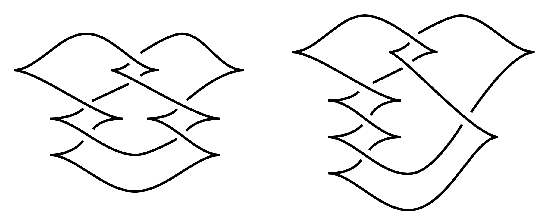
Legendrian contact homology proved to be a powerful invariant of Legendrian submanifolds. For Legendrian knots in \( \mathbb{R}^3 \), LCH is a “nonclassical” invariant: that is, it can distinguish between Legendrian knots that share their classical invariants (smooth knot type, Thurston–Bennequin number, and rotation number). Building off of his classification of Legendrian unknots discussed in Section 2, Eliashberg (unpublished) proposed a family of Legendrian knots with the same classical invariants that could be distinguished through their LCH: Whitehead doubles of Legendrian unknots, where the unknots have the same Thurston–Bennequin number but different rotation numbers. Topologically, these Whitehead doubles are called twist knots. In [e9], Chekanov provided the first rigorous proof that there is a pair of Legendrian knots with the same classical invariants but different LCH. This pair is of topological knot type \( m(5_2) \) and is shown in Figure 4; like Eliashberg’s family, the Chekanov pair are twist knots. Shortly thereafter, Epstein, Fuchs, and Meyer [e6] used Chekanov’s techniques to show that Eliashberg’s entire family of twist knots can be distinguished through their LCH invariants.
In the decades since its introduction by Eliashberg and collaborators, Legendrian contact homology has firmly established itself as a central concept in modern contact and symplectic topology. Among other things, LCH has contributed to structural results about Legendrian knots, such as the classification of Legendrian twist knots mentioned in Section 2; it has been extended to a filtered invariant in the realm of quantitative symplectic geometry; it has been used to study Legendrian submanifolds in higher dimensions than knots, and to develop invariants of smooth knots; it has provided Arnold-type lower bounds on the number of Reeb chords of Legendrian submanifolds; it has led to surgery formulas for symplectic homology on Weinstein domains; and it has figured prominently in the theory of wrapped Fukaya categories and Liouville sectors. LCH has also provided strong and surprising bridges between symplectic topology and many other areas of mathematics, including microlocal sheaf theory, cluster theory, and topological string theory. A full treatment of these developments is far beyond the scope of this article, but the interested reader might consult [e22] for a survey of results about LCH in the specific setting of Legendrian knots in \( \mathbb{R}^3 \).
We close this section by noting one particular line of current research that has direct roots in Eliashberg’s original work on LCH from the 1990s. Given a contact manifold \( V \), one can construct a category whose objects are Legendrian submanifolds of \( V \) and whose morphisms are certain cobordisms in the symplectization \( V\times\mathbb{R} \) called exact Lagrangian cobordisms. By design and as outlined in [8] by Eliashberg, Givental, and Hofer, SFT is meant to be functorial. What this means for LCH is that an exact Lagrangian cobordism between two Legendrians should induce a map between the Chekanov–Eliashberg dg algebras of the Legendrians, and that this map should be invariant under Hamiltonian isotopy of the cobordism. This was demonstrated for Legendrian knots in \( V=\mathbb{R}^3 \) by Ekholm, Honda, and Kálmán [e20] about a decade ago. Consequently, one can approach the problem of classifying exact Lagrangian cobordisms with fixed ends by studying the induced cobordism map on LCH. This remains an active area of research.
4. Ruling invariants
In the mid-1980s, Eliashberg [1] proved that the group of symplectomorphisms of a symplectic manifold is \( C^0 \) closed in the group of diffeomorphisms, a foundational result in symplectic topology that essentially says that symplectic topology exists as a field. While the significance of this result will be discussed elsewhere in this volume, of importance here is Eliashberg’s self-described “combinatorial” proof technique. His proof relies on the existence of a combinatorial decomposition of front diagrams of certain Legendrian submanifolds into simple pieces, and the persistence of such a decomposition under regular homotopy starting from the 0-section of a 1-jet bundle of a manifold. Eliashberg also applied the decomposition technique in [1], [2] to prove results about symplectic, Lagrangian, and Legendrian embeddings.
The success of Eliashberg’s front decomposition idea inspired several mathematicians to formalize such decompositions into an invariant of Legendrian knots called a ruling. Ruling invariants have played a fundamental role in defining nonclassical Legendrian invariants distinct from, but related to, those arising from SFT, in making connections between different types of Legendrian invariants, and in linking Legendrian and smooth knot theory.
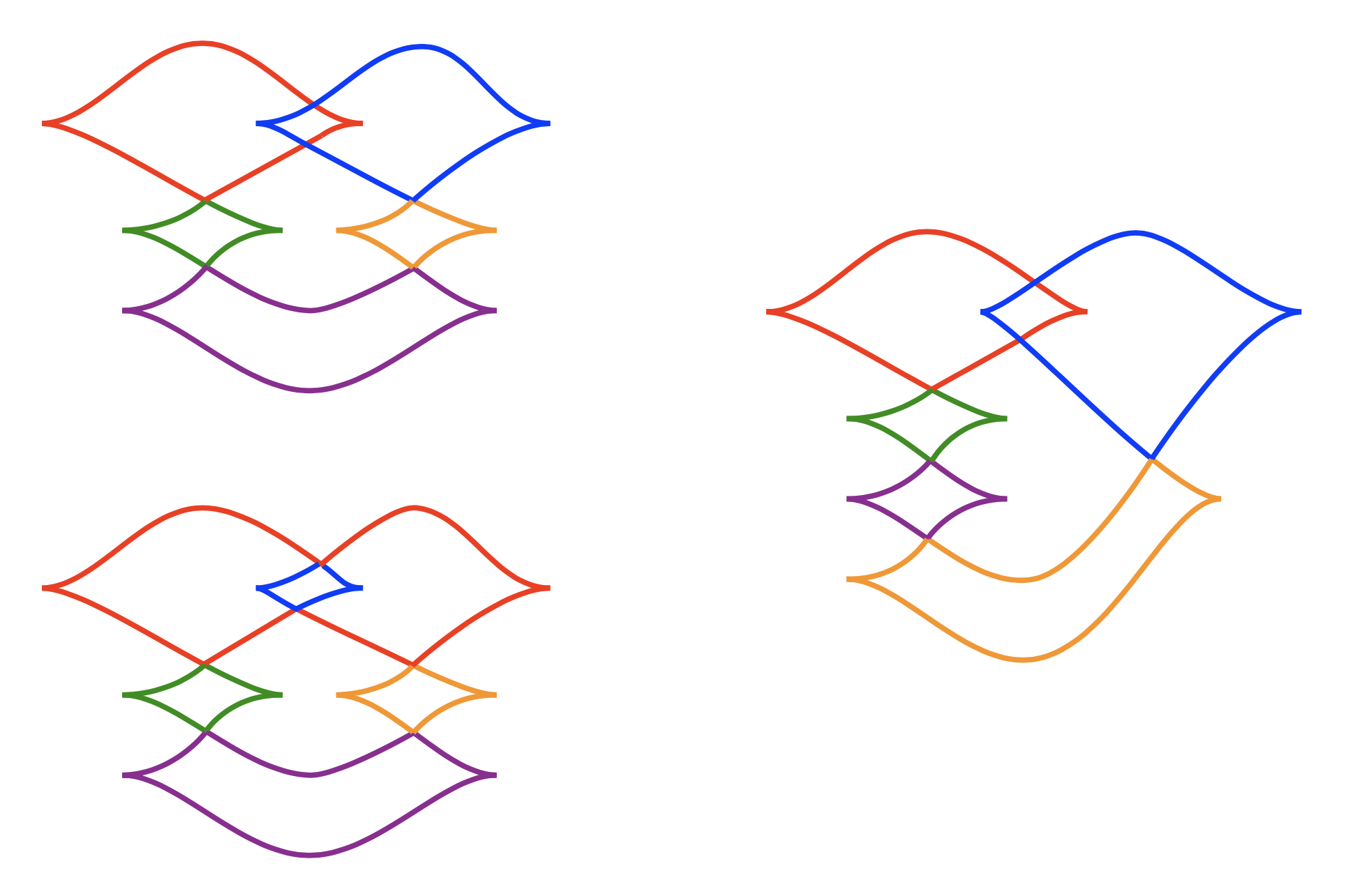
Roughly speaking, a ruling of a Legendrian knot \( \Lambda \) in \( \mathbb{R}^3 \) is a decomposition of its front diagram into “eyes” with prescribed combinatorics near points where the boundary of an eye switches from one strand of the front diagram to another; see Figure 5 and the recent survey [e21]. In particular, the boundary of an eye can switch only if the crossing of the front is “graded” in some sense and only if the eyes involved are either nested or disjoint near the switch. The set of graded rulings is a Legendrian invariant, and may be encoded by a “ruling polynomial” [e12]. The graded ruling polynomial is a strong enough invariant to distinguish Chekanov’s pair of \( m(5_2) \) knots in Figure 4. As was the case for Eliashberg’s original work, rulings have geometric applications. For example, Chekanov and Pushkar applied rulings to prove Arnold’s 4-cusp conjecture, namely that every Legendrian isotopy between the inward- and outward-pointing fibers of \( ST^*\mathbb{R}^2 \) has an intermediate Legendrian with four cusps in its projection to the base \( \mathbb{R}^2 \) [e12].
Another early success of ruling invariants was their connection to Legendrian contact homology. A useful method for extracting computable invariants from the Chekanov–Eliashberg DGA is to look at its 1-dimensional representations, called augmentations. Geometrically, augmentations are closely connected with exact Lagrangian fillings of Legendrian knots (i.e., cobordisms from the empty set). Fuchs built on Eliashberg’s decomposition idea to independently define rulings, and used them to prove that the existence of a ruling implies the existence of an augmentation [e11]; the converse is also true. This connection continues to be an active area of research, both in terms of understanding how counts of augmentations and rulings are related and in generalizing the relationship to higher-dimensional representations of the Chekanov–Eliashberg DGA.
Legendrian contact homology is not the only point of connection between rulings and other Legendrian invariants. From the beginning (cf. ([1], §3) and [e12]), rulings were viewed as combinatorial shadows of the theory of generating families of Legendrian submanifolds. Notably, Fuchs and Rutherford proved that, in fact, every ruling comes from a generating family [e18]. Eliashberg’s influence on the theory of generating families and its applications is discussed in greater detail elsewhere in this volume.
As with other ideas discussed in this essay, Eliashberg’s ideas related to rulings have inspired a large and still expanding body of subsequent work by many other mathematicians. This work not only encompasses the theory of Lagrangian cobordisms between Legendrians discussed in the previous section, but also extends beyond symplectic topology to incorporate relations to subjects such as microlocal sheaves and cluster algebras.
Lenhard Ng is a Professor of Mathematics at Duke University, and works in symplectic and contact geometry and low-dimensional topology. As a postdoc from 2001 to 2006 at the Institute for Advanced Study and Stanford University, he was supervised by Yasha Eliashberg.
Joshua Sabloff is the J. McLain King 1928 Professor of Mathematics at Haverford College. His research lies in contact, symplectic, and low-dimensional topology. He was a student of Yasha Eliashberg at Stanford, and earned a PhD under Yasha’s supervision in 2002.
