by Frédéric Bourgeois
1. Introduction
In order to describe the context in which contact homology was born, it is useful to go back to the origins of a whole collection of symplectic and contact invariants. Holomorphic curves were introduced in symplectic geometry by Gromov [e1], in the case of closed symplectic manifolds \( (W, \omega) \). These are maps \( u : \Sigma \to W \) defined on a Riemann surface \( \Sigma \) with complex structure \( j \) satisfying the Cauchy–Riemann equation \[ du \circ j = J \circ du \] for a compatible almost complex structure \( J \) on \( W \), i.e., an endomorphism \( J \) of \( TW \) satisfying \( J^2 = -I \) as well as the compatibility conditions
- \( \omega(J \cdot\,, J \cdot\,) = \omega(\,\cdot\,, \cdot\,) \),
- \( \omega(v, Jv) > 0 \) for all nonzero tangent vectors \( v \) to \( W \).
Sometimes the first condition is omitted, and we then say that our almost complex structure \( J \) is tame.
Originally, such maps \( u \) were referred to as pseudoholomorphic, because the compatible almost complex structure \( J \) is generally not integrable, i.e., one cannot find complex local coordinates on \( W \) so that \( J \) corresponds to the multiplication by \( i \) in these coordinates. As mathematicians became used to these objects with time, the name \( J \)-holomorphic became fashionable. Nowadays, one can simply refer to these maps as “holomorphic” if the context is clear. This last simplification may even be due to Yasha Eliashberg’s pleas during various conferences and lectures, where he has insisted with an evident sense of humor that the prefixes “pseudo-” or “\( J \)-” suggest that these maps are not as good as actual holomorphic ones, while in fact they are perfectly fine, and that this terminology is “degrading our field”. He even suggested calling these maps “Gromomorphic” but for some reason it seems that this name was never used in the literature.
In a nutshell, the fact that moduli spaces of \( J \)-holomorphic curves can lead to symplectic invariants mainly rests on two key facts. First, the set of compatible almost complex structures on a symplectic manifold \( (W, \omega) \) is contractible. In particular, any symplectic manifold can be equipped with such a compatible almost complex structure. Moreover, different choices of compatible almost complex structures are always isotopic, and different isotopies between fixed compatible almost complex structures are themselves isotopic, and so on.
Second, the moduli spaces of \( J \)-holomorphic curves can be compactified by adding nodal curves, i.e., Riemann surfaces with pairs of points identified to each other and called nodes, as well as \( J \)-holomorphic maps from these Riemann surfaces to \( W \) that are compatible with these identifications. This is the content of the celebrated Gromov compactness theorem in symplectic geometry. In particular, intersection numbers in these compactified moduli spaces are well defined and can be used in the construction of symplectic invariants. In some cases, these intersections numbers are the symplectic invariants themselves; this is the case for Gromov–Witten invariants. In other situations, these intersection numbers are used as coefficients in a differential of a chain complex, which is defined in such a way that its homology is a symplectic invariant; this is the case of Floer homology. For the latter type of theory, nodal curves are replaced with broken trajectories in the compactification of moduli spaces. The simplest type of broken trajectory consists of two cylinders, such that the end of the first one coincides with the beginning of the second one.
Some might say that Floer homology is not strictly speaking an invariant based on holomorphic curves, since the corresponding differential counts solutions of the so-called Floer equation, which is an inhomogeneous Cauchy–Riemann equation, involving a Hamiltonian function in its right-hand side. But as explained in paragraph 1.4.C\( ^{\prime} \) of [e1], the graph of a map satisfying such an inhomogeneous Cauchy–Riemann equation is \( \widetilde{J} \)-holomorphic for a suitable choice of almost complex structure \( \widetilde{J} \) on the target space of this graph. Yasha indeed insists that it is very useful to read the whole of Gromov’s original article [e1] as it contains many fruitful ideas. More specifically, this interpretation of Floer trajectories as holomorphic maps is explained in Section 2.2 of [5] using the notion of a stable Hamiltonian structure. All this is a beautiful illustration of one of Yasha’s mottos: “Look at graph” — which is fundamental in an impressive number of situations within contact and symplectic topology.
When \( (W, \omega) \) is a symplectic manifold with boundary, satisfying some type of convexity property near its boundary, holomorphic curves obey a maximum principle, hence they are confined in a compact region of the target manifold \( W \), and the corresponding moduli spaces are still compact. This is, for example, the case of symplectic manifolds \( (W, \omega) \) with contact-type boundary \( (\partial W = M, \xi) \), for which there exists near \( \partial W \) a Liouville vector field \( v \), i.e., \( \mathcal{L}_v \omega = \omega \), such that \( v \) is transverse to \( \partial W \) and pointing outside \( W \). In that case, the kernel of the 1-form \( \alpha = \imath(v) \omega \) is a contact structure \( \xi \). In other words, the 1-form \( \alpha \) satisfies the property that \( \alpha \wedge (d\alpha)^{n-1} \) does not vanish wherever it is defined, and is called a contact form. Different choices \( v_1 \) and \( v_2 \) of a vector field as above lead to different contact structures, but the collection of all convex combinations of \( v_1 \) and \( v_2 \) leads to an isotopy between the corresponding contact structures, and by Gray’s stability theorem for closed contact manifolds, these contact structures are actually diffeomorphic.
Some beautiful instances of successful applications of holomorphic curves in this type of symplectic manifolds \( (W, \omega) \) are described by Yasha in [2]. There, holomorphic maps are defined over the disc and its boundary must be mapped to a given submanifold of \( (W, \omega) \) satisfying appropriate conditions. The development of these techniques were followed by an impressive number of further developments. Those are described in another chapter of this volume [e76]. A more recent theory relying on holomorphic curves in such \( (W, \omega) \) is symplectic homology, which is a version of Floer homology using a Hamiltonian function and a compatible almost complex structure having an appropriate asymptotic behavior near \( \partial W \).
In a symplectic manifold \( (W, \omega) \) with contact type boundary, any sufficiently small open neighborhood of \( \partial W = M \) can be symplectically embedded in the symplectization of \( (M, \xi) \). The latter is the manifold \( \mathbb{R} \times M \) equipped with the symplectic form \( d(e^t \alpha) \), where \( t \) is a global coordinate on the \( \mathbb{R} \) factor and \( \alpha \) is a contact form for \( \xi \). Note that this symplectic manifold does not depend on the choice of \( \alpha \). Yasha used to explain to his students that, for some time, symplectizations were considered by experts to be bad manifolds to work with holomorphic curves. This is because the lower end of a symplectization (with \( t \) very small) is concave, as the Liouville vector field \( \frac{\partial}{\partial t} \) is pointing inside the manifold, instead of being convex. Therefore, holomorphic curves are allowed to sink deeply into this lower end and visit an unbounded region of the manifold, so that the corresponding moduli spaces will not be compact. This all changed when Hofer [e2] understood the behavior of finite energy holomorphic curves at infinity of a symplectization, when equipped with a compatible almost complex structure with an appropriate behavior outside a compact set. This will be detailed below, but for now let us just say that near each end of a symplectization, such holomorphic curves are asymptotic to cylinders over periodic orbits of a distinguished vector field in the contact manifold.
Symplectizations are often schematically represented as cones, since the symplectic volume tends to zero as \( t \to -\infty \). But then, when drawing a holomorphic curve sinking into the negative end of a symplectization, it gets impossible to see what happens to it as the picture becomes arbitrarily small. Maybe this partially explains why the behavior of holomorphic curves symplectizations was not understood before Hofer’s breakthrough work. In a public address during the first Yashafest conference at Stanford in 2007, Alexander Givental astutely observed with a lot of humor that Yasha’s vision of mathematics is so great because he is very small. What this really means, he explained, is that Yasha imagines mathematical objects as being much larger than himself, so that he can visualize all their details and develop a good intuition. This is obvious for anyone who has had the chance to discuss mathematics with Yasha on a sidewalk terrace, where it would be typical for him to describe a huge holomorphic cylinder, say, coming from the other side of the street and illustrate with it some new idea that had crossed his mind. Coming back to symplectizations, it is a better idea to draw them as cylinders, so that one can see more clearly what happens to holomorphic curves at their negative end.
Shortly after the work of Hofer, Yasha and he envisioned how to adapt ideas from Floer homology to symplectizations: this was the birth of contact homology. Yasha described contact homology in the proceedings of his invited lecture at the ICM 1998 in Berlin [3]. As we shall see below, this theory was geometrically and algebraically more complex than Floer theory, but this did not stop them from developing an even more general theory. With Givental, they introduced Symplectic Field Theory (SFT) [4], which can be thought of as the general framework for using holomorphic curves of arbitrary topology in symplectic manifolds with convex and concave ends. SFT is also described in an article by Yasha in the proceedings of the ICM 2006 in Madrid [7]. This very general theory is the subject of another chapter in this volume [e77].
One of the more general features of full SFT in comparison with contact homology is that a pair of holomorphic curves seen as a broken configuration may be glued along an arbitrary number of pairs of cylindrical ends, instead of along a single pair of ends. This additional complexity plays an important role in the description of the relevant compactified moduli spaces, as well as in the algebraic formalism of the theory. During the second SFT Workshop in Leipzig in 2006, Yasha gave many lectures on SFT formalism. In order to illustrate this more sophisticated gluing for holomorphic curves in this context, he repeatedly made the following gesture. He placed one hand with its fingers pointing up below the other hand with its fingers pointing down, so that matching fingertips would figure pairs of cylindrical ends that could potentially be glued to each other, and in order to convey the fact that gluing was optional for each pair, he wiggled all his fingers with his hands in this position. In order to answer most questions from audience members puzzled by SFT, Yasha would repeat the same gesture. This eventually prompted a desperate cry by Viktor Ginzburg from the back of the amphitheater: “Yasha, define something!” As a testimony to Yasha’s generosity, a special session was added to the program at Yasha’s request so that he could explain in more detail these puzzling aspects of SFT. This session lasted until so late at night that the gates outside the building were locked, and all participants (including Yasha himself) had to climb over the wall in order to leave the campus.
Since the author cannot wiggle his fingers in front of the reader, a few things will be defined in Sections 2 and 3, concerning holomorphic curves in symplectizations and the contact homology algebra, respectively, in the hope that readers will be able to comprehend the applications of contact homology explained in Section 4.
2. Holomorphic curves in symplectizations
In this section, we describe geometric constructions in the symplectization of a contact manifold, leading to the definition of a suitable class of holomorphic curves for our purposes. We then outline the analysis required to construct the moduli spaces of such holomorphic curves with the necessary geometric properties in view of the definition of homological invariants.
2.1. Closed Reeb orbits
Let \( (M, \xi) \) be a closed contact manifold of dimension \( 2n-1 \). To any contact form \( \alpha \) for \( \xi \), one can associate its Reeb vector field \( R_\alpha \), characterized by the property that it spans the one-dimensional kernel of \( d\alpha \): \( \imath(R_\alpha) \,d\alpha = 0 \), and by the normalization condition \( \alpha(R_\alpha) = 1 \). Although this vector field strongly depends on the choice of \( \alpha \), the collection of Reeb fields for a given contact structure shares important dynamical properties.
Of particular interest are the periodic orbits of such a vector field. Let \( \gamma : \mathbb{R}/T\mathbb{Z} \to M \) be a closed Reeb orbit of period \( T \): \( \dot{\gamma}(t) = R_\alpha(\gamma(t)) \). In other words, if we denote the flow of \( R_\alpha \) by \( (\varphi^\alpha_t)_{t \in \mathbb{R}} \), we have \( \varphi^\alpha_T(\gamma(0)) = \gamma(0) \). Since \( \mathcal{L}_{R_\alpha} \alpha = 0 \), this flow preserves the contact structure, and we can restrict \( d\varphi^\alpha_T \) to \( \xi_{\gamma(0)} \). The closed Reeb orbit \( \gamma \) is said to be nondegenerate if this restriction does not have 1 as an eigenvalue. It can be shown that for a generic choice of \( \alpha \), all closed Reeb orbits are nondegenerate; in this case, the contact form \( \alpha \) is said to be nondegenerate. We denote by \( \mathcal{P}_\alpha \) the collection of all periodic orbits of the Reeb field \( R_\alpha \) modulo reparametrization shift, and for any \( T > 0 \) we denote by \( \mathcal{P}^{\le T}_\alpha \) the subset of closed orbits with period less than or equal to \( T \). For a nondegenerate contact form \( \alpha \), the set \( \mathcal{P}^{\le T}_\alpha \) is finite for all \( T > 0 \), and the set \( \mathcal{P}_\alpha \) is at most countable.
To any nondegenerate closed Reeb orbit \( \gamma \), given a symplectic trivialization \( \mathcal{F} \) of \( \gamma^*\xi \), one can associate its Conley–Zehnder index \( \mu_{CZ}(\gamma, \mathcal{F}) \in \mathbb{Z} \). Intuitively, this index measures the twisting of the Reeb flow around the closed orbit \( \gamma \), relative to the chosen trivialization \( \mathcal{F} \). Any other symplectic trivialization \( \mathcal{F}^{\prime} \) can be obtained by acting on \( \mathcal{F} \) with a loop of symplectic matrices \( P : \mathbb{R}/T\mathbb{Z} \to \mathrm{Sp}(2n-2) \). A natural identification of \( \pi_1(\mathrm{Sp}(2n-2)) \) with \( \mathbb{Z} \) is obtained by retracting a loop in \( \mathrm{Sp}(2n-2) \) to \( \mathrm{U}(n-1) \), then taking its complex determinant with values in \( S^1 \subset \mathbb{C} \) and considering the degree of the resulting map from \( S^1 \) to itself. In particular, to the above loop \( P \) one can associate in this way its Maslov index \( \mu(P) \in \mathbb{Z} \). It then turns out that \[ \mu_{CZ}(\gamma, \mathcal{F}^{\prime}) = \mu_{CZ}(\gamma, \mathcal{F}) + 2 \mu(P). \] It follows that the Conley–Zehnder index depends only on the homotopy class of the chosen trivialization, and that its parity does not depend on it at all.
Note that there is a consistent way of obtaining symplectic trivializations for all orbits in \( \mathcal{P}_\alpha \) from a minimal number of choices (see for example Section 2.1 of [e28]), but we shall not use this here in order to keep the exposition more elementary. Instead, let us choose once and for all a symplectic trivialization for each \( \gamma \in \mathcal{P}_\alpha \), and denote its Conley–Zehnder index with respect to this chosen trivialization by \( \mu_{CZ}(\gamma) \).
Let \( \gamma \) be a closed Reeb orbit with minimal period \( T \), i.e., the map \( \gamma : [0, T) \to M \) is injective. We can consider its multiples \[ \gamma^{(m)} : \mathbb{R}/mT\mathbb{Z} \to M : t \mapsto \gamma(t \textrm{ mod } T), \] for all integers \( m \ge 1 \). We say that a closed Reeb orbit is bad if it is of the form \( \gamma^{(m)} \) and if \( \mu_{CZ}(\gamma^{(m)}) \) and \( \mu_{CZ}(\gamma^{(1)}) \) have different parities; otherwise, we say that it is good. Note that bad orbits are necessarily of even multiplicity \( m \), and that if \( \gamma^{(m)} \) is bad for some \( m \), then all orbits of the form \( \gamma^{(2k)} \) are bad for all \( k \). We define by \( \mathcal{P}^\mathrm{ g}_\alpha \) the subset of good closed Reeb orbits for the Reeb vector field corresponding to the contact form \( \alpha \).
2.2. Holomorphic curves
Consider the symplectization \( (\mathbb{R} \times M, d(e^t \alpha)) \) of our contact manifold, where \( t \) is a global coordinate on \( \mathbb{R} \). Note that the symplectomorphism class of this manifold does not depend on the choice of the contact form \( \alpha \) for \( \xi \). Choose an almost complex structure \( J \) on this symplectization, i.e., an endomorphism of the tangent bundle of \( \mathbb{R} \times M \) such that \( J^2 = -I \), and satisfying the following properties:
- \( J \) preserves \( \xi \) and \( J |_\xi \) is compatible with the symplectic form \( d\alpha \), in the sense that \[ d\alpha(Jv,Jw) =d\alpha(v,w) \] for all tangent vectors \( v, w \) in \( \xi \), and \( d\alpha(v,Jv) > 0 \) for all nonzero tangent vectors \( v \) in \( \xi \);
- \( J \frac{\partial}{\partial t} = R_\alpha \);
- \( J \) is invariant by translation in the \( \mathbb{R} \)-direction.
The first two conditions imply that \( J \) is compatible with the symplectic structure \( \omega = d(e^t \alpha) \). Like on closed symplectic manifolds, the space \( \mathcal{J}(M,\alpha) \) of such almost complex structures is contractible.
Consider the Riemann sphere \( \mathbb{C}\mathrm{P}^1 \) equipped with its natural complex structure \( j \), as well as distinct points (called punctures) \( x_1, \dots, x_q \in \mathbb{C}\mathrm{P}^1 \) with \( q \ge 0 \). Given a map \[ u : \Sigma_u = \mathbb{C}\mathrm{P}^1 \setminus \{ x_1, \dots, x_q \} \to \mathbb{R} \times M \] defined on the punctured Riemann surface \( \Sigma_u \), we denote by \( u_\mathbb{R} \) and \( u_M \) its components in \( \mathbb{R} \) and in \( M \), respectively. Such a map is said to be \( J \)-holomorphic if \( du \circ j = J \circ du \). The Hofer energy of \( u \) is defined as \[ E(u) = \sup_{\phi \in \mathcal{C}} \int_{\Sigma_u} u^*d(\phi \alpha), \] where \( \mathcal{C} = \{ \phi \in C^\infty(\mathbb{R}, [0,1] \ | \ \phi^{\prime}(t) \ge 0 \} \). This is a substitute for the symplectic area with respect to the symplectic form \( d(e^t \alpha) \), which would be infinite if \( u \) approached the positive end of the symplectization. Another interesting quantity is the so-called area of \( u \), defined by \[ A(u) = \int_{\Sigma_u} u^* \,d\alpha. \] Note that since \( J \) is compatible with \( d(e^t \alpha) \) and \( J |_\xi \) is compatible with \( d\alpha \), the Hofer energy and the area are nonnegative: \( E(u) \ge 0 \) and \( A(u) \ge 0 \) for any holomorphic map \( u \). Moreover, if \( E(u)=0 \), then \( u \) is a constant map, and if \( A(u)=0 \), then the image of \( u_M \) is contained in a Reeb trajectory.
It turns out that any proper holomorphic map \( u \) with finite Hofer energy, i.e., \( E(u) < \infty \), has a precise behavior near each of its punctures. If \( p \) denotes a puncture of \( \Sigma_u \), the module and argument of a local complex coordinate for \( \mathbb{C}\mathrm{P}^1 \) centered on \( p \) determine polar coordinates \( (\rho, \theta) \) near \( p \). Then we have \[ \lim_{\rho \to 0} u_\mathbb{R}(\rho, \theta) = \pm \infty \quad\text{ and }\quad \lim_{\rho \to 0} u_M(\rho, \theta) = \gamma(\mp T\theta/2\pi), \] for some \( \gamma \in \mathcal{P}_\alpha \) of period \( T \). In this case, we say that the map \( u \) is asymptotic to \( \gamma \) at \( \pm \infty \) and that the corresponding puncture \( p \) is positive (resp. negative).
The prescribed asymptotic behavior of such maps near the \( q \) punctures is specified by a list \( \Gamma \) of \( q \) periodic orbits in \( \mathcal{P}_\alpha \). By convention, the asymptotes corresponding to positive punctures are listed first, and are separated by a semicolon from the asymptotes corresponding to negative punctures that are listed afterwards. Two holomorphic maps \( u \) and \( u^{\prime} \) with the same asymptotic behavior \( \Gamma \) are said to be equivalent, which will be denoted by \( u \sim u^{\prime} \), if there exists a biholomorphism \( h : \Sigma_u \to \Sigma_{u^{\prime}} \) such that \( u^{\prime} \circ h = u \). The equivalence class of a holomorphic map \( u \) will be denoted by \( [u] \).
The set of equivalence classes of holomorphic maps with a given asymptotic behavior \( \Gamma \) will be denoted by \( \widetilde{\mathcal{M}}(\Gamma) \). As this set actually parametrizes the solutions of partial differential equation modulo reparametrization, it deserves to be called a moduli space. Elements of this moduli space can be given a homology class in \( H_2(M, \mathbb{Z}) \) after some appropriate choices have been fixed for all closed orbits in \( \mathcal{P}_\alpha \). This moduli space can then be decomposed as a disjoint union of smaller moduli spaces according to these homology classes (see, for example, Section 2.2 of [e28]). Again, we shall not make such choices here in order to keep the exposition more elementary.
Since the almost complex structure \( J \) was chosen to be \( \mathbb{R} \)-invariant on the symplectization, the above moduli spaces are equipped with an \( \mathbb{R} \)-action: for any \( \tau \in \mathbb{R} \), we set \( \tau \cdot [u_\mathbb{R}, u_M] = [u_\mathbb{R} + \tau, u_M] \) for each equivalence class \( [u] = [u_\mathbb{R}, u_M] \) in some of these moduli spaces. The fixed points of this \( \mathbb{R} \)-action are easily identified as the vertical cylinders over periodic orbits in \( \mathcal{P}_\alpha \). This corresponds to a very particular choice of asymptotic behavior \( \Gamma = (\gamma ; \gamma) \), with one positive and one negative puncture each corresponding to the same closed orbit \( \gamma \) of period \( T \). In that case, it follows from Stokes theorem that for any \( [u] \in \widetilde{\mathcal{M}}(\Gamma) \), we have \( A(u) = T - T = 0 \) so that the above \( \mathbb{R} \)-action is trivial. Except in this very special case of moduli spaces consisting of trivial cylinders, this \( \mathbb{R} \)-action is therefore free. We then consider the corresponding quotient \( \widetilde{\mathcal{M}}(\Gamma)/\mathbb{R} = \mathcal{M}(\Gamma) \). In the case of trivial cylinders, we simply set \( \mathcal{M}(\gamma;\gamma) = \widetilde{\mathcal{M}}(\gamma;\gamma) \).
Before turning to the properties of these moduli spaces \( \mathcal{M}(\Gamma) \), let us specify the particular type of holomorphic curves which will be of interest in order to define contact homology. As sketched in Section 1, contact homology can be thought of as the simplest theory for holomorphic curves adapting the ideas from Floer homology to symplectizations. Our aim is therefore to limit ourselves to the simplest possible types of holomorphic curves. Note that in the above discussion, we already restricted ourselves to rational curves. A first naive choice would be to further restrict ourselves to holomorphic cylinders, like in Floer homology where only Floer trajectories parametrized by \( \mathbb{R} \times S^1 \) are counted in order to define the differential. In the case of symplectizations, this would correspond to holomorphic curves with one positive and one negative puncture. However, this simple approach does not work in general, for the following reason. In order to construct invariants out of moduli spaces, it is essential to consider and understand their compactifications. In our situation, we have to understand the compactification \( \overline{\mathcal{M}}(\Gamma) \) of our moduli spaces \( \mathcal{M}(\Gamma) \), using compactness results from [5]. Roughly speaking, this compactification is obtained by adding to \( \mathcal{M}(\Gamma) \) the so-called holomorphic buildings, consisting of several (but finitely many) levels. Each level contains one or more holomorphic curves in a symplectization, so that its positive asymptotes coincide with the negative asymptotes from the level directly above it, and its negative asymptotes coincide with the positive asymptotes from the level directly below it. The topmost level has positive asymptotes \( \Gamma^+ \) and the bottommost level has negative asymptotes \( \Gamma^- \), such that \( \Gamma = (\Gamma^+ ; \Gamma^-) \). In particular, the compactification \( \overline{\mathcal{M}}(\Gamma) \) of a moduli space \( \mathcal{M} (\Gamma) \) consisting of holomorphic cylinders could contain holomorphic buildings with two levels, the top level containing a pair of pants, i.e., a holomorphic curve with one positive and two negative punctures, and the bottom level containing two holomorphic curves: a holomorphic cylinder and a holomorphic plane, i.e., a holomorphic curve with just one positive puncture. Note that this is just the simplest possible situation involving more general holomorphic curves than simply holomorphic cylinders, but we shall see later that it is of particular importance. For general contact manifolds, such holomorphic buildings can occur, so that it is not possible to work with compact moduli spaces consisting of holomorphic buildings involving holomorphic cylinders only. Instead, one has to find a more general class of holomorphic curves so that the corresponding compactified moduli spaces will solely consist of holomorphic buildings involving holomorphic curves in the same class. If this class of holomorphic curves contains holomorphic cylinders, then it must also contain tree-like holomorphic curves, i.e., holomorphic curves with exactly one positive puncture, but with an arbitrary number of negative punctures, as shown by the above example with more than one holomorphic plane in the bottom level. On the other hand, the compactification of moduli spaces of tree-like holomorphic curves cannot involve holomorphic curves with more than one positive puncture. If this were the case, the corresponding holomorphic building would need to contain at least one holomorphic curve \( u \) without positive puncture but with at least one negative puncture. But such a holomorphic map \( u \) cannot exist, because by Stokes theorem, the area \( A(u) \) of this map would be negative, which is forbidden.
The above discussion explains why, for the purpose of defining contact homology, we shall require that our holomorphic maps \( u \) have exactly one positive puncture and an arbitrary number \( r \ge 0 \) of negative punctures. Their asymptotic behavior will be of the form \( \Gamma = (\gamma^+ ; \gamma^-_1, \dots, \gamma^-_r) \), where \( \gamma^+ \in \mathcal{P}_\alpha \) has period \( T^+ \) and \( \gamma^-_i \in \mathcal{P}_\alpha \) has period \( T^-_i \) for \( i= 1, \dots, r \). If the moduli space \( \mathcal{M}(\gamma^+ ; \gamma^-_1, \dots, \gamma^-_r) \) is nonempty, then by Stokes theorem \( 0 \le A(u) = T^+ - \sum_{i=1}^r T^-_i \) with equality if and only if \( r=1 \) and \( \gamma^+ = \gamma^-_1 \).
2.3. Moduli spaces of tree-like holomorphic curves
Let us now turn to the properties of the moduli spaces \( \mathcal{M}(\gamma^+ ; \gamma^-_1, \dots, \gamma^-_r) \) of tree-like curves. In this section, we will refer to the original articles for various facets in the study of these moduli spaces, though most of these topics are covered in the very comprehensive lectures by Wendl [e62]. The local structure of these moduli spaces can be studied using tools from functional analysis and, more specifically, Fredholm theory. Our moduli space is seen as a subset of a larger configuration space, consisting of all maps \( u \) defined on a sphere with \( r+1 \) punctures and satisfying the asymptotic conditions corresponding to \( (\gamma^+ ; \gamma^-_1, \dots, \gamma^-_r) \). In order to make use of Fredholm theory, this configuration space must be equipped with a suitable Banach structure, and the standard choice is to require our maps to satisfy some Sobolev regularity. The minimal choice is to require one weak derivative, since the Cauchy–Riemann equation has order 1. For the Sobolev regularity to make sense for maps between manifolds, these maps must be at least continuous, and for the Sobolev embedding theorem to apply for our maps \( u \) defined on surfaces, we must work with exponent \( p > 2 \). This leads to \( W^{1,p} \)-type Sobolev spaces. Note that if one prefers to work in the Hilbert case \( p=2 \), one can instead require two weak derivatives and use \( W^{2,2} \)-type Sobolev spaces instead. This latter choice was made in the literature corresponding to some other variants of contact homology, but here we will keep to the first choice, so that our configuration space \( \mathcal{B} = \mathcal{B}(\gamma^+ ; \gamma^-_1, \dots, \gamma^-_r) \) will be a Banach manifold modeled on a \( W^{1,p} \) space.
Let us specify the measure of the punctured sphere which is used to define the Sobolev norm. In Floer theory, one uses the standard measure \( ds \, d\theta \) on the cylinder \( \mathbb{R} \times S^1 \) with coordinates \( (s,\theta) \). It is therefore natural in the case of a punctured sphere \( \mathbb{C}\mathrm{P}^1 \setminus \{ x_1, \dots, x_q \} \) to use a measure that coincides with \( ds \, d\theta \) on the punctured neighborhoods \( \mathbb{R}^- \times S^1 \) of \( x_1, \dots, x_q \) with coordinates \( (s, \theta) = (\log \frac{\rho}{\rho_0}, \theta) \), where \( (\rho, \theta) \) are the polar coordinates used in Section 2.2 and \( \rho < \rho_0 \) in these neighborhoods. There is however a complication in the case of symplectizations, as compared to that of Floer theory. Despite the fact that closed Reeb orbits are assumed to be nondegenerate (which is a statement about the linearized return map restricted to \( \xi \)), the linearized return map along a closed orbit in the whole tangent space \( T(\mathbb{R} \times M) \) of the symplectization has an eigenvalue 1 with, as corresponding eigenspace, the plane spanned by the Reeb vector field \( R_\alpha \) and the Liouville vector field \( \frac{\partial}{\partial t} \). In other words, nondegenerate closed Reeb orbits, seen as Hamiltonian periodic orbits in the symplectization \( \mathbb{R} \times M \), are degenerate in the sense of Floer theory. This will cause some analytic complications, and in order to avoid these it is necessary that we add exponential weights to our measure near the punctures, and use the measure \( e^{d|s|} \,ds \, d\theta \) in the corresponding neighborhoods. The corresponding Sobolev space with one weak derivative and exponent \( p \) are the referred to as a \( W^{1,p,d} \) space. It can be shown that holomorphic maps \( u \) with finite Hofer energy will converge with exponential speed to vertical cylinders over closed Reeb orbits near the punctures; see [e5] for estimates in dimension three and Appendix A of [5] for the setting to generalize these to higher dimensions. More precisely, in the above \( (s,\theta) \) coordinates around a puncture where \( u_\mathbb{R} \to \pm\infty \), there exists a closed Reeb orbit \( \gamma \), as well as constants \( s_0 \in \mathbb{R} \) and \( \theta_0 \in \mathbb{R}/2\pi\mathbb{Z} \) such that \begin{equation} \label{eq:expconv1} | u_\mathbb{R} (s,\theta) \pm T(s - s_0)| \le C e^{-d|s|} \tag{2.1} \end{equation} and \begin{equation} \label{eq:expconv2} d_M(u_M(s,\theta), \gamma(\mp T(\theta-\theta_0)/2\pi)) \le C e^{-d|s|}, \tag{2.2} \end{equation} using some auxiliary distance \( d_M \) in \( M \), for \( C > 0 \) sufficiently large and \( d > 0 \) sufficiently small. Therefore, the configuration space \( \mathcal{B} \) defined using a \( W^{1,p,d} \) space will contain the holomorphic curves we are interested in and is a suitable choice for constructing in it the desired moduli space.
Note that, in Equations \eqref{eq:expconv1} and \eqref{eq:expconv2}, the constants \( s_0 \) and \( \theta_0 \) depend on the map \( u \in \mathcal{B} \). Because of this, the tangent space \( T_u \mathcal{B} \) will not only consist of sections of \( u^*T(\mathbb{R} \times M) \) that are in \( W^{1,p,d} \), but also of sections which converge near punctures to nonvanishing vectors in the plane spanned by the Reeb field \( R_\alpha \) and the Liouville field \( \frac{\partial}{\partial t} \). Therefore, in addition to a \( W^{1,p,d} \) space of sections of \( u^*T(\mathbb{R} \times M) \), the tangent space \( T_u \mathcal{B} \) will also contain a two-dimensional summand for each puncture, spanned by sections supported in a neighborhood of the puncture and taking the constant value \( R_\alpha \) or \( \frac{\partial}{\partial t} \) in a smaller neighborhood of the puncture. The total dimension of these extra summands in \( T_u \mathcal{B} \) is \( 2q \), where \( q \) is the number of punctures. The norm of these special sections will be determined by the asymptotic value at the corresponding puncture via an auxiliary metric on \( \mathbb{R} \times M \).
In additional to these two-dimensional summands, the tangent space \( T_u \mathcal{B} \) will also contain a finite dimensional summand corresponding to the change of position for the punctures in \( \mathbb{C}\mathrm{P}^1 \). Each puncture introduces two degrees of freedom, but the quotient by action of biholomorphisms of \( \mathbb{C}\mathrm{P}^1 \), acting transitively on triplets of points in \( \mathbb{C}\mathrm{P}^1 \), reduces these degrees of freedom by 6, so we obtain \( 2(q-3) \) degrees of freedom corresponding to the position of the \( q \) punctures.
For a map \( u\in\mathcal{B} \), the expression \( du - J \circ du \circ j \) is a \( (0,1) \)-form with \( L^p \) regularity on the domain of \( u \) with values in \( u^*T(\mathbb{R} \times M) \). One therefore reinterprets the Cauchy–Riemann equation as a section of a Banach bundle \( \mathcal{E} \to \mathcal{B} \) with fibers \( \mathcal{E}_u \) that are modeled on an \( L^{p,d} \) space of suitable vector-valued \( (0,1) \)-forms over the configuration space \( \mathcal{B} \). The moduli space is then realized as the zero set \( s^{-1}(0) \) of such a section \( s \). In the case of a finite rank vector bundle over a finite dimensional manifold, it suffices to show that the section is sufficiently regular and is a submersion along its zero set in order to show that \( s^{-1}(0) \) is a manifold of a given dimension. In the above Banach setting, the regularity condition on \( s \) is replaced by the Fredholm property: the vertical differential \( D_u : T_u \mathcal{B} \to \mathcal{E}_u \) of \( s \) at some map \( u \), which is a linear, bounded operator between Banach spaces, should have a finite dimensional kernel, a closed image and a cokernel, i.e., the quotient of its target space by its image, of finite dimension as well. In that case, the Fredholm index of \( D \) defined as \[ \operatorname{ind} D_u = \dim \ker D_u - \dim \operatorname{coker} D_u \] is locally constant on the space of Fredholm operators. In our case, it will depend only on the combinatorial data decorating the moduli space under consideration, so that it does not depend on \( u \in \mathcal{B} \). Furthermore, if the differential of \( s \) is surjective along \( s^{-1}(0) \), then this zero locus is a smooth manifold of finite dimension given by \( \operatorname{ind} D_u \). This Fredholm index for a Cauchy–Riemann type operator on a Riemann surface can be computed via the Riemann–Roch theorem, which says that the index of a Cauchy–Riemann operator on sections of a vector bundle of complex rank \( n \) and of first Chern class \( c_1 \) over a closed Riemann surface of genus \( g \) is given by \( n(2-2g) + 2c_1 \). There are several ways to compute the index of \( D_u \), but here is the author’s favorite approach. First, restrict the operator \( D_u \) to the \( W^{1,p,d} \) part of its domain, or, in other words, remove from its domain the summands of total dimension \( 4q -6 \) corresponding to the variations of \( s_0 \) and \( \theta_0 \) in Equations \eqref{eq:expconv1} and \eqref{eq:expconv2}, as well as the positions of the punctures. Second, conjugate the restricted operator with the multiplication by a function of the form \( e^{d|s|} \) near each puncture, so that the resulting operator is defined in a \( W^{1,p} \) space and takes its values in an \( L^p \) space. While the original operator has the form \( D_u \zeta = \partial_s \zeta + J_0 \partial_\theta \zeta + A_j(s, \theta) \zeta \) near puncture \( j \), in a suitable trivialization of \( u^*T(\mathbb{R} \times M) \), the conjugated operator will have a similar form with the matrix \( A_j \) replaced with \( \tilde{A}_j = A_j - \varepsilon_j d I \) where \( \varepsilon_j \) is the sign of the puncture \( j \), with \( j = 1, \dots, q \). Near the punctures, such operators are exactly of those encountered as the linearization of the Floer equation in symplectic geometry. One can show Theorem 3.2.12 of [e4] that the index of these operators is additive under the gluing operation at one or several punctures. The trick is then to glue two identical operators along corresponding pairs of punctures, using a suitable clutching function for the vector bundle at each puncture so that the expressions of the operators match in the regions that are to be identified when gluing the Riemann surfaces. The glued Riemann surface has genus \( q-1 \) and the vector bundle over it has its first Chern class given by \( \sum_{j=1}^q \varepsilon_j \mu_{CZ}(\tilde{A}_j) \), where \( \varepsilon_j \) is the sign of the puncture \( j \). By the Riemann–Roch theorem, this glued operator has index \[ n(2-2(q-1)) + 2 \sum_{j=1}^q \varepsilon_j \mu_{CZ}(\tilde{A}_j), \] and by the additivity of the index, this is twice the index of the conjugated operator. A simple calculation shows that \( \mu_{CZ}(\tilde{A}_j) = \mu_{CZ}(A_j) - \varepsilon_j \), so that the index of the restricted operator can be expressed as \[ n(2-q) - q + \sum_{j=1}^q \varepsilon_j \mu_{CZ}(A_j). \] Adding the removed degrees of freedom, the index of \( D_u \) is given by \[ n(2-q) + 3q - 6 + \sum_{j=1}^q \varepsilon_j \mu_{CZ}(A_j). \] Since the \( q \) punctures correspond to one positive puncture and \( r \) negative punctures, and the indices \( \mu_{CZ}(A_j) \) for \( j = 1 , \dots, q \) are given by \( \mu_{CZ}(\gamma^+) \) and \( \mu_{CZ}(\gamma^-_i) \) for \( i = 1, \dots, r \), we finally obtain \begin{equation} \label{eq:index} \operatorname{ind} D_u = (n-3)(1-r) + \mu_{CZ}(\gamma^+) - \sum_{i=1}^r \mu_{CZ}(\gamma^-_i).\tag{2.3} \end{equation} This formula gives the dimension of the moduli space \( \widetilde{\mathcal{M}}(\gamma^+ ; \gamma^-_1, \dots, \gamma^-_r) \), provided one can ensure that the operator \( D_u \) is surjective for all \( [u] \) in this moduli space.
Under this surjectivity assumption, one can construct a gluing map with a sufficiently large parameter \( R > 0 \) which is defined over any compact subset of \( \widetilde{\mathcal{M}}(\Gamma_1) \times \widetilde{\mathcal{M}}(\Gamma_2) \), where the last negative asymptote of \( \Gamma_1 \) coincides with the positive asymptote of \( \Gamma_2 \). This map takes its values in \( \widetilde{\mathcal{M}}(\Gamma) \), where \( \Gamma \) has the same positive asymptote as \( \Gamma_1 \), and its negative asymptotes are the negative asymptotes of \( \Gamma_1 \) (except the last one) and the negative asymptotes of \( \Gamma_2 \). This map takes a pair of holomorphic curves \( (u_1, u_2) \) to a holomorphic curve \( u_R \) that nearly coincides with \( (u_{1, \mathbb{R}} + R, u_{1,M}) \) on \( \mathbb{R}^+ \times M \) and with \( (u_{2,\mathbb{R}} -R, u_{2,M}) \) on \( \mathbb{R}^- \times M \). When the positive asymptote of \( \Gamma_2 \) is a closed Reeb orbit covering \( m \) times a simple closed orbit, there are \( m \) different ways of gluing \( u_1 \) and \( u_2 \), differing by a shift by any multiple \( 2\pi/m \) of the coordinate \( \theta \) near the positive puncture of \( u_2 \) before identification of this coordinate with an analogous coordinate near the last negative puncture of \( u_1 \). This combinatorial choice must be specified as part of the gluing data for the moduli spaces \( \widetilde{\mathcal{M}}(\Gamma_1) \) and \( \widetilde{\mathcal{M}}(\Gamma_2) \). The construction of this gluing map follows the same strategy as other uses of holomorphic curves in contact and symplectic geometry, but relies on the specific Banach structures for contact homology that are described above. One first constructs a preglued map \( \tilde{u}_R \) which is constructed from the maps \( u_1 \) and \( u_2 \) using cutoff functions near their common asymptote. Then one applies an infinite dimensional version of the implicit function theorem to find a holomorphic curve \( u_R \) near \( \tilde{u}_R \) in the configuration space \( \mathcal{B}(\Gamma) \). The application of this theorem requires three estimates. First, the \( L^{p,d} \) norm of \( d\tilde{u}_R - J \circ d\tilde{u}_R \circ j \) must tend to 0 as \( R \to \infty \). Second, the operator \( D_{\tilde{u}_R} \) must have a right inverse which is uniformly bounded in \( R \), with respect to the Banach norms described above. Third, the second order term in the Taylor expansion of the section \( s : \mathcal{B} \to \mathcal{E} \) around \( \tilde{u}_R \) must be bounded uniformly in \( R \) with respect to the same norms. The second estimate is typically the most delicate one to establish. To this end, one first constructs an approximate right inverse \( Q_R \) for \( D_{\tilde{u}_R} \) using bounded right inverses for \( D_{u_1} \) and \( D_{u_2} \), this is where the surjectivity assumption mentioned above is essential. More precisely, one has to prove that the norm of the operator \( D_{\tilde{u}_R} \circ Q_R - I \) tends to 0 as \( R \to \infty \). Then, standard arguments provide an actual right inverse with the desired properties for \( R \) sufficiently large. Once this gluing map is defined, it can be used to construct the compactification of the moduli spaces of holomorphic curves as a smooth manifold with boundaries and corners. Indeed, it turns out that holomorphic buildings with \( \ell \) levels constitute a codimension \( \ell - 1 \) submanifold in the boundary of the compact moduli space of holomorphic buildings.
In order to define orientations having suitable properties with respect to the above gluing map on our moduli spaces, it is necessary to work in a more abstract setting. Let \( \mathcal{O} = \mathcal{O}(\gamma^+ ; \gamma^-_1, \dots, \gamma^-_r) \) be the space of differential operators which are of the same form as the above operators \( D_u \) with \( u \in \mathcal{B} \). In particular, all \( D \in \mathcal{O} \) are Fredholm operators with the same index as above. Although the dimensions of the vector spaces \( \ker D \) and \( \operatorname{coker} D \) can vary as \( D \) varies in \( \mathcal{O} \), the real lines \( \Lambda^{\max} \ker D \otimes \Lambda^{\max} (\operatorname{coker} D)^* \) naturally fit together to form a real line bundle \( \mathcal{L} \to \mathcal{O} \), called a determinant line bundle; this is true for general spaces of Fredholm operators; see the Appendix of [e3]. An orientation of \( \mathcal{L} \) is equivalent to the data of a nonvanishing section of \( \mathcal{L} \). Such a section exists if and only if \( \mathcal{L} \) is a trivial vector bundle. Note that \( \mathcal{O} \) is homotopy equivalent to a product of \( q=r+1 \) circles, because of the possible values of \( \theta_0 \in \mathbb{R}/2\pi\mathbb{Z} \) in Equation \eqref{eq:expconv2}. It turns out that \( \mathcal{L} \) is trivial along a circle factor corresponding to a puncture where \( D \) has the asymptotic behavior for the asymptote \( \gamma \) if and only if \( \gamma \) is a good orbit ([e16], Theorem 3). This is the reason for the distinction between good and bad orbits in Section 2.1. If we restrict ourselves to good orbits as asymptotes of holomorphic curves, then these considerations guarantee that all moduli spaces are orientable. One can then construct [e16] a coherent set of orientations for the determinant line bundles corresponding to all operator spaces \( \mathcal{O}(\Gamma) \). Here the word “coherent” means that these orientations are preserved by the gluing maps \( \mathcal{L}(\Gamma_1) \otimes \mathcal{L}(\Gamma_2) \to \mathcal{L}(\Gamma) \) induced by the gluing of operators in a similar way as the gluing map for holomorphic curves discussed above. These coherent orientations are uniquely determined by choices of orientations for the determinant line bundles with a single (positive) asymptote at all good closed Reeb orbits. One subtle point is that the coherent orientation on \( \mathcal{L}(\gamma^+; \gamma^-_1, \dots, \gamma^-_r) \) also depends on the ordering of the negative asymptotes. This can be understood by the following considerations: gluing the above coherent orientation successively with the coherent orientations on \( \mathcal{L}(\gamma^-_i) \) for \( i= r, \dots, 1 \), one obtains the coherent orientation on \( \mathcal{L}(\gamma^+) \). But the coherent orientation on \( \mathcal{L}(\gamma^-_r) \otimes \dots \otimes \mathcal{L}(\gamma^-_1) \) depends on the ordering of the oriented bases for the kernel and cokernel of operators in \( \mathcal{O}(\gamma^-_i) \) for \( i = r, \dots, 1 \). Permuting two consecutive asymptotes \( \gamma^-_i \) and \( \gamma^-_{i+1} \) will change the product orientation exactly when both permuted bases consist of an odd number of vectors, or in other words when the Fredholm indices \eqref{eq:index} of the corresponding operators \( \mu_{CZ}(\gamma^-_i)+n-3 \) and \( \mu_{CZ}(\gamma^-_{i+1})+n-3 \) are both odd. Pulling back this system of coherent orientations on the determinant line bundles by the map \( \widetilde{\mathcal{M}}(\Gamma) \to \mathcal{O}(\Gamma) : u \mapsto D_u \) gives a coherent system of orientations on the moduli spaces \( \widetilde{\mathcal{M}}(\Gamma) \). In the case of a surjective operator \( D_u \), its determinant line is indeed given by \( \Lambda^\mathrm{ max}(\ker D_u) \), where \( \ker D_u \) is naturally identified with the tangent space \( T_u\widetilde{\mathcal{M}}(\Gamma) \). Note that this system of coherent orientations is defined for all moduli spaces, regardless of their dimensions. In addition to this, one can define canonical orientations for all moduli spaces \( \widetilde{\mathcal{M}}(\Gamma) \) of dimension one. These are defined by pushing forward the natural orientation of the real line by the \( \mathbb{R} \)-action on \( \widetilde{\mathcal{M}}(\Gamma) \). Then all one-dimensional moduli spaces are equipped with two orientations: the coherent one and the canonical one. Each connected component of \( \widetilde{\mathcal{M}}(\Gamma) \), or equivalently each element \( [u] \) of \( \mathcal{M}(\Gamma) \), can therefore be equipped with a sign: \( +1 \) if both orientations agree, and \( -1 \) otherwise.
The above construction of the moduli spaces \( \mathcal{M}(\Gamma) \) as oriented finite dimensional manifolds relies on the assumption that the operator \( D_u \) is surjective for every \( [u] \in \mathcal{M}(\Gamma) \). In other theories involving holomorphic curves in contact and symplectic topology, this property is achieved using so-called classical transversality techniques [e14], which consist in choosing the almost complex structure \( J \) generically. However, these methods fail in the presence of multiply covered holomorphic curves, or, in other words, holomorphic curves that factor though a ramified covering of Riemann surfaces. Such covering can unavoidably occur, for example, in the case of a moduli space \( \mathcal{M}(\gamma) \) of holomorphic planes with a single positive puncture asymptotic to a closed Reeb orbit \( \gamma \) which is the iterate of another closed Reeb orbit. Several other methods have been developed to overcome these very delicate technical difficulties. Most of them consist in perturbing the right-hand side of the Cauchy–Riemann equation. When multiply covered holomorphic curves arise, these come with a nontrivial group of automorphisms, and it is typically impossible to achieve transversality of the section \( s : \mathcal{B} \to \mathcal{E} \) with the zero section at such curves using an equivariant right-hand side. For this reason, it is necessary to used so-called multivalued perturbations, or, in other words, a finite set of right-hand sides for the Cauchy–Riemann equation which is globally preserved by the automorphism group. When this set consists of more than one element, it is important not to overcount holomorphic curves, so that the perturbations, as well as the corresponding elements in the perturbed moduli space, have to carry fractional weights so that the sum of all relevant weights remains equal to 1. This is why the count \( n(\Gamma) \) of elements in a perturbed zero-dimensional moduli space \( \mathcal{M}(\Gamma) \) is a rational number, as each element comes both with a sign coming from the orientations and with a fractional weight coming from the necessary perturbation to achieve transversality. When no such perturbation is required, \( n(\Gamma) \in \mathbb{Q} \) is the sum over all elements \( [u] \in \mathcal{M}(\Gamma) \) of the sign of \( [u] \) divided by the order of the automorphism group of \( u \).
Beyond this very brief description of the perturbation scheme for our moduli spaces, the complete constructions are extremely long and difficult to describe in great detail. Over the years, many different research teams have developed their own approach to this very complicated problem. The theory of polyfolds introduced by Hofer, Wysocki and Zehnder [e65] aims to frontally attack all analytical problems in order to produce moduli spaces that are as close as possible to honest manifolds with boundaries and corners. Kuranishi structures were used by Fukaya and Ono [e6] in the context of Gromov–Witten invariants and these may be used for contact homology in order to obtain suitable moduli spaces. In the same spirit, Bao and Honda [e68] used semiglobal Kuranishi charts to provide a definition of the contact homology algebra. Hutchings and Nelson [e50], [e67] used automatic transversality techniques to define contact homology in dimension three. Pardon [e49], [e61] developed an algebraic, rather than geometric, approach via virtual fundamental cycles, in order to define suitable counts of elements in low-dimensional moduli spaces, and applied this technique to define contact homology in full generality.
3. Contact homology algebra
In this section, we introduce the algebraic framework that mirrors the geometric properties of the moduli spaces of holomorphic curves and leads to the definition of homological invariants for contact manifolds, namely contact homology and its variants.
3.1. Differential graded algebra
Since the moduli spaces of holomorphic curves from Section 2.2 are decorated with closed Reeb orbits, it is necessary to make these orbits part of the algebraic formalism that will incorporate the count of elements in these moduli spaces. To each closed orbit \( \gamma \in \mathcal{P}^\mathrm{ g}_\alpha \), we associate a formal generator \( q_\gamma \), in order to distinguish geometric objects from algebraic ones. The generator \( q_\gamma \) will be given a grading obtained by looking at the dimension formula for moduli spaces of holomorphic curves. We set \( |q_\gamma| = \mu_{CZ}(\gamma) + n - 3 \), so that in view of Equation \eqref{eq:index} we have \begin{equation} \label{eq:dim} \dim \mathcal{M}(\gamma^+; \gamma^-_1, \dots, \gamma^-_r) = |q_{\gamma^+}| - \sum_{i=1}^r |q_{\gamma^-_i}| -1.\tag{3.1} \end{equation}
Let \( \mathcal{A} \) be the supercommutative, graded, unital algebra generated by \( q_\gamma \) for all \( \gamma \in \mathcal{P}^\mathrm{ g}_\alpha \)
over some ring \( \mathcal{R} \). We are working here with an algebra, and not a module as in Floer theory, because our holomorphic curves are
allowed to have several negative asymptotes (i.e., when \( r > 1 \)), and in this case we will be using the formal expression
\( q_{\gamma^-_1} \dots q_{\gamma^-_r} \). Moreover, we need a unital algebra so that the unit \( 1 \in \mathcal{A} \) can be used when there are
no negative asymptotes (i.e., when \( r = 0 \)). In the above definition,
“supercommutative” means that for any pair of elements \( a, b \in \mathcal{A} \)
with pure grading (so that \( |a| \) and \( |b| \) are well defined), we have \( a b = (-1)^{|a| |b|} b a \). This rule is introduced in order to mirror the
behavior of the coherent orientations of the moduli spaces \( \mathcal{M}(\gamma^+; \gamma^-_1, \dots, \gamma^-_r) \) under the exchange
of two orbits \( \gamma^-_i \) and \( \gamma^-_j \).
Let us now discuss the possible choices for the ring \( \mathcal{R} \). Making the choice \( \mathcal{R} = \mathbb{Z}/2\mathbb{Z} \) would eliminate all sign considerations, but such coefficients are incompatible with the signed and weighted counts of elements in moduli spaces, which are rational numbers, as explained in Section 2.3. Therefore, the simplest choice is to take \( \mathcal{R} = \mathbb{Q} \), under our assumption that \( c_1(\xi)=0 \). When this assumption is not satisfied, a more elaborate choice of ring is required if we wish to retain a grading in our algebraic formalism. One then usually chooses \( \mathcal{R} = \mathbb{Q}[H_2(M)] \). A general element of this group ring has the form \( \sum_{A \in H_2(M)} q_A e^A \), where \( q_A \in \mathbb{Q} \) and \( e^A \) is a formal generator with grading \( |e^A| = -2 \langle c_1(\xi), A \rangle \). Once again, this grading is chosen in view of the dimension formula for the moduli spaces of holomorphic curves. Note that the grading of \( \mathcal{R} \) is even, so that it does not interfere with the supercommutativity property of \( \mathcal{A} \). Of course, one can make this choice \( \mathcal{R} = \mathbb{Q}[H_2(M)] \) even in the case where \( c_1(\xi)=0 \), and, more generally, one can choose \( \mathcal{R} \) to be any graded algebra over the graded ring \( \mathbb{Q}[H_2(M)] \). Such special choices can be useful in certain situations.
Let us now turn to the definition of the differential \( \partial : \mathcal{A} \to \mathcal{A} \). We require \( \partial \) to be a linear superderivation of degree \( -1 \) of \( \mathcal{A} \), or, in other words, \( \partial (\lambda a+ \mu b) = \lambda \partial a + \mu \partial b \) for all \( a, b \in \mathcal{A} \), \( \lambda, \mu \in \mathcal{R} \), and \( |\partial a | = |a|-1 \) as well as \( \partial(ab) = (\partial a)b + (-1)^{|a|} a \partial b \) for all \( a, b \in \mathcal{A} \) of pure grading. The differential is therefore characterized by its value on the generators of \( \mathcal{A} \), and we define \begin{equation} \label{eq:d} \partial q_{\gamma^+} = m_{\gamma^+} \sum_{r \ge 0} \sum_{\substack{\{\gamma^-_1, \dots, \gamma^-_r\} \subset \mathcal{P}^g_\alpha \\ |q_{\gamma^-_1}| + \dots + |q_{\gamma^-_r}| = |q_{\gamma^+}|-1}} n(\gamma^+;\gamma^-_1, \dots, \gamma^-_r) \ q_{\gamma^-_1} \dots q_{\gamma^-_r},\tag{3.2} \end{equation} where \( m_{\gamma^+} \) is the multiplicity of the orbit \( \gamma^+ \) and \( n(\gamma^+;\gamma^-_1, \dots, \gamma^-_r) \in \mathbb{Q} \) is the signed and weighted count of the elements \( [u] \) in the moduli space \( \mathcal{M}(\gamma^+;\gamma^-_1, \dots, \gamma^-_r) \), as described in Section 2.3. Note that this sum makes sense because our definition of the grading in \( \mathcal{A} \) in terms of the dimension formula for the moduli spaces guarantees that the moduli spaces involved in this sum are zero-dimensional, and hence finite by compactness. Also note that, in view of the supercommutativity rule in \( \mathcal{A} \) mimicking the behavior of coherent orientations for moduli spaces, the above expression is well defined independently of the ordering of the generators \( q_{\gamma^-_1}, \dots, q_{\gamma^-_r} \).
It then follows from the same philosophy as in Morse or Floer theory, using the properties of the moduli spaces of holomorphic curves, that we have the identity \( \partial \circ \partial = 0 \). In other words, \( (\mathcal{A}, \partial) \) is a differential graded algebra (DGA). More precisely, this is proved by considering the boundary of one-dimensional moduli spaces \( \mathcal{M}(\gamma^+;\gamma^-_1, \dots, \gamma^-_r) \). The signed weighted count of the elements in this boundary then corresponds to the coefficient of \( q_{\gamma^-_1} \dots q_{\gamma^-_r} \) in the expression \( \partial \circ \partial q_{\gamma^+} \). But the sum of the weights associated to elements in the boundary of a connected component of the above one-dimensional moduli space vanishes by definition of the weights and of the signs. This implies that \( \partial \circ \partial q_{\gamma^+} = 0 \) for any generator \( q_{\gamma^+} \).
The homology \( \ker \partial / \operatorname{im} \partial \) of the DGA \( (\mathcal{A}, \partial) \) is a graded algebra; it is called the contact homology of \( (M, \xi) \) and is denoted by \( CH(M,\xi) \). This terminology and this notation are justified by the fact that, unlike the DGA \( (\mathcal{A}, \partial) \), contact homology does not depend on the various choices made during this construction, in particular the contact form \( \alpha \) for \( \xi \) and the compatible complex structure \( J \) on \( (\xi, d\alpha) \).
The proof of the invariance property of contact homology is similar in philosophy to the proof of \( \partial \circ \partial = 0 \). The main difference lies in the fact that we are not considering holomorphic curves in a symplectization anymore, but in a symplectic cobordism of the form \( (\mathbb{R} \times M, d(e^t \alpha_t)) \), with \( \alpha_t \) interpolating very slowly between different choices of contact forms: \( \alpha_t = \alpha_+ \) for \( t \) sufficiently large, and \( \alpha_t = \alpha_- \) for \( t \) sufficiently small. Furthermore, the fact that \( \alpha_t \) varies slowly with \( t \) guarantees that the 2-form \( d(e^t \alpha_t) \) is nondegenerate, hence symplectic. This symplectic cobordism is also equipped with a compatible almost complex structure that depends on \( t \) and interpolates between a compatible almost complex structure \( J_+ \) for the symplectization of \( \alpha_+ \) and a compatible almost complex structure \( J_- \) for the symplectization of \( \alpha_- \). Different discrete choices can also be made at the ends of this cobordism in order to define the corresponding DGAs \( (\mathcal{A}_+, \partial_+) \) and \( (\mathcal{A}_-, \partial_-) \) via their respective symplectizations.
The properties of the moduli spaces of holomorphic curves in such a symplectic cobordism are very similar to those in the case of a symplectization, except for the fact that they are not equipped with a free action of \( \mathbb{R} \) by translation along the first coordinate of the cobordism. Therefore, the dimension formula for these moduli spaces does not contain the final \( -1 \) term as in Equation \eqref{eq:dim}, and the count of elements in zero-dimensional moduli spaces will lead to the definition of a map of degree 0 instead of \( -1 \). This map \( \Phi : (\mathcal{A}_+, \partial_+) \to (\mathcal{A}_-, \partial_-) \) is defined to be a morphism of unital algebras, in other words, \( \Phi(1) = 1 \), \( \Phi(\lambda a + \mu b) = \lambda \Phi(a) + \mu \Phi(b) \) and \( \Phi(ab) = \Phi(a) \Phi(b) \) for all \( a, b \in \mathcal{A}_+ \) and \( \lambda, \mu \in \mathcal{R} \). This map is then also characterized by its value on generators \( q_{\gamma^+} \) of \( \mathcal{A}_+ \), and a formula similar to Equation \eqref{eq:d} is used to define \( \Phi(q_{\gamma^+}) \).
The boundary of one-dimensional moduli spaces of holomorphic curves in the above symplectic cobordism consists of holomorphic buildings with two levels, one in the cobordism and one in the symplectization of \( \alpha_+ \) or of \( \alpha_- \). Therefore, the vanishing weighted count of the elements in this boundary leads to the identity \( \Phi \circ \partial_+ = \partial_- \circ \Phi \). In other words, \( \Phi \) is a unital DGA map and induces a map \( \overline{\Phi} \) between the homologies of \( (\mathcal{A}_+, \partial_+) \) and \( (\mathcal{A}_-, \partial_-) \). It remains to show that this induced map is actually an isomorphism.
Exchanging the roles of \( (\mathcal{A}_+, \partial_+) \) and \( (\mathcal{A}_-, \partial_-) \), and reversing the sign of \( t \) in the interpolations \( \alpha_t \) and \( J_t \), one obtains similarly a unital DGA map \( \Psi : (\mathcal{A}_-, \partial_-) \to (\mathcal{A}_+, \partial_+) \) inducing a map \( \overline{\Psi} \) between the homologies of \( (\mathcal{A}_-, \partial_-) \) and \( (\mathcal{A}_+, \partial_+) \). A gluing argument then shows that the composition \( \overline{\Psi} \circ \overline{\Phi} \) is induced by the concatenation of both interpolations, which is isotopic to the constant interpolation between \( (\alpha_+, J_+) \) and itself. Note that this constant interpolation induces the identity maps on \( (\mathcal{A}_+, \partial_+) \) and on its homology, because the moduli spaces that are zero-dimensional without taking the quotient by the \( \mathbb{R} \)-action on the first coordinate of the symplectization consist purely of vertical cylinders over closed Reeb orbits. If one could show that the map induced in homology by an interpolation as above is invariant under isotopy of such interpolations, then we could deduce that \( \overline{\Psi} \circ \overline{\Phi} \) is the identity. Similarly, \( \overline{\Phi} \circ \overline{\Psi} \) would also be the identity, so that \( \overline{\Phi} \) would be an isomorphism as desired.
Given an isotopy of interpolations between interpolations inducing unital DGA maps \[ \Phi_0, \Phi_1 : (\mathcal{A}_+, \partial_+) \to (\mathcal{A}_-, \partial_-), \] we can construct a one-parameter family of symplectic cobordisms of the form \( (\mathbb{R} \times M, d(e^t \alpha_{t,\sigma})) \) equipped with compatible almost complex structures \( J_\sigma \), for \( \sigma \in [0,1] \). We consider the moduli space \( \mathcal{M}^\sigma(\gamma^+;\gamma^-_1, \dots, \gamma^-_r) \) of holomorphic curves in this family of cobordisms, consisting of all pairs \( (\sigma, [u_\sigma]) \) where \( \sigma \in [0,1] \) and \( u_\sigma \) is a \( J_\sigma \)-holomorphic map in \( (\mathbb{R} \times M, d(e^t \alpha_{t,\sigma})) \). By the compactness theorem for holomorphic curves in symplectic cobordisms, the zero-dimensional moduli spaces \( \mathcal{M}^\sigma \) are finite, so that only finitely many values \( \sigma_1, \dots, \sigma_N \in [0,1] \) appear as the first coordinate of an element in such a moduli space. If \( N=0 \), then the boundary elements of one-dimensional moduli spaces \( \mathcal{M}^\sigma \) must be of the form \( (0, [u_0]) \) or \( (1,[u_1]) \), so that \( \Phi_0 = \Phi_1 \). We can therefore concentrate on small intervals around the special values \( \sigma_i \) for \( i= 1, \dots, N \) or, in other words, assume that \( N=1 \). A \( (\Phi_0, \Phi_1) \)-derivation \( K : \mathcal{A}_+ \to \mathcal{A}_- \) is a map satisfying \( K(1) = 0 \), \[ K(\lambda a + \mu b) = \lambda K(a) + \mu K(b) \quad\text{for all } a, b \in \mathcal{A} \] and \( \lambda, \mu \in \mathcal{R} \), and \[ K(q_1 \dots q_k) = \sum_{g \in S_k} \sum_{j=1}^k (-1)^{|q_{g(1)} \dots q_{g(j-1)}|} \Phi_0(q_{g(1)} \dots q_{g(j-1)}) K(q_{g(j)}) \Phi_1(q_{g(j+1)} \dots q_{g(k)}), \] for all generators \( q_1, \dots, q_k \) of \( \mathcal{A}_+ \), where \( S_k \) denotes the permutation group of \( \{ 1, \dots, k \} \). We define \( K(q_{\gamma^+}) \) by a formula similar to Equation \eqref{eq:d} using the signed and weighted count of elements in the zero-dimensional moduli spaces \( \mathcal{M}^\sigma(\gamma^+;\gamma^-_1, \dots, \gamma^-_r) \). Since the parameter \( \sigma \in [0,1] \) provides an additional degree of freedom in comparison with the previous situation, the dimension formula for these moduli spaces has a final term \( +1 \) instead of \( -1 \) in Equation \eqref{eq:dim}, so that \( |q_{\gamma^+}| = |q_{\gamma^-_1} \dots q_{\gamma^-_r}| - 1 \) and \( K \) is of degree \( +1 \) as announced.
We then study the compactification of the one-dimensional moduli space \( \mathcal{M}^\sigma(\gamma^+;\gamma^-_1, \dots, \gamma^-_r) \) using a suitable perturbation scheme. When a sequence of holomorphic curves degenerates into a holomorphic building with 2 levels, which necessarily occurs when \( \sigma \to \sigma_1 \), it is necessary to arrange the perturbation scheme so that each connected component in the level corresponding to the family of symplectic cobordism has its own value of \( \sigma \) very close to \( \sigma_1 \). Only the component counted by \( K \) has \( \sigma = \sigma_1 \), while the other components have either \( \sigma < \sigma_1 \), so that it is counted by \( \Phi_0 \), or \( \sigma > \sigma_1 \), so that it is counted by \( \Phi_1 \). With a perturbation scheme that averages over all the possible inequalities, the count of elements in the boundary of the one-dimensional moduli space \( \mathcal{M}^\sigma(\gamma^+;\gamma^-_1, \dots, \gamma^-_r) \) leads to the identity \( \Phi_1 - \Phi_0 = K \circ \partial_+ + \partial_- \circ K \). It follows that the induced maps on homology coincide: \( \overline{\Phi}_0 = \overline{\Phi}_1 \).
3.2. Cylindrical contact homology
Since the differential graded algebra in the previous section is quite large and its homology can be difficult to compute, it can be convenient to insist on working with holomorphic cylinders only in order to obtain an invariant which is simpler to compute. Of course, this will be possible only under suitable conditions.
If our holomorphic curves have a single negative puncture, the output of the differential will be a linear combination of generators corresponding to closed Reeb orbits, so that it is not necessary to use the algebra \( \mathcal{A} \) anymore. Using the same type of ring \( \mathcal{R} \) as in the previous section, let \( C^\mathrm{ cyl} \) be the graded \( \mathcal{R} \)-module freely generated by \( q_\gamma \) for all \( \gamma \in \mathcal{P}^\mathrm{ g}_\alpha \).
We define the cylindrical differential \( \partial^\mathrm{ cyl} : C^\mathrm{ cyl} \to C^\mathrm{ cyl} \) as the linear map of degree \( -1 \) characterized by \[ \partial^\mathrm{ cyl} q_{\gamma^+} = m_{\gamma^+} \sum_{\substack{\gamma^- \in \mathcal{P}^g_\alpha \\ |q_{\gamma^-}| = |q_{\gamma^+}|-1}} n(\gamma^+;\gamma^-) \ q_{\gamma^-}. \] In other words, in the definition \eqref{eq:d} of the contact homology differential, we restrict ourselves to the term \( r=1 \) corresponding to holomorphic cylinders.
The arguments from the previous section to show that \( \partial^\mathrm{ cyl} \circ \partial^\mathrm{ cyl} = 0 \) can be adapted to holomorphic cylinders provided a one-parameter family of holomorphic cylinders can only degenerate into a level two holomorphic building with a cylinder in each level. However, there can a priori be another possible configuration for such a level two holomorphic building: a pair of pants with one positive puncture and two negative punctures in the upper level, and a plane with one positive puncture together with a vertical cylinder in the lower level. In order to prevent the existence of such a configuration, it suffices to forbid the existence of a closed Reeb orbit that can play the role of a positive asymptote for a rigid holomorphic plane. In view of the dimension formula \eqref{eq:dim}, we need to assume that there is no contractible \( \gamma \in \mathcal{P}^\mathrm{ g}_\alpha \) such that \( \mu_{CZ}(\gamma) + n - 3 = 1 \). Under this condition, it is possible to define cylindrical contact homology \( CH^\mathrm{ cyl}(M, \xi) \) as the homology of the chain complex \( (C^\mathrm{ cyl}, \partial^\mathrm{ cyl}) \).
Similarly, the arguments from the previous section to show invariance of contact homology can be adapted to the cylindrical case if rigid holomorphic planes cannot exist in symplectic cobordisms or in one-parameter families of symplectic cobordisms. Due to the dimension shifts of the corresponding moduli spaces as in the previous section, we need to assume that there is no contractible \( \gamma \in \mathcal{P}^\mathrm{ g}_\alpha \) such that \( \mu_{CZ}(\gamma) + n - 3 \) is equal to 0 or to \( -1 \).
We can summarize the above discussion as follows: if that there is no contractible \( \gamma \in \mathcal{P}^\mathrm{ g}_\alpha \) such that \( \mu_{CZ}(\gamma) + n - 3 \) is equal to \( +1 \), to 0 or to \( -1 \), then cylindrical contact homology \( CH^\mathrm{ cyl}(M, \xi) \) is well defined and is an invariant of the contact manifold \( (M, \xi) \). Note that more restrictive conditions were sometimes used in the literature to guarantee the existence of this contact invariant, when it was still an open problem to achieve transversality for the moduli spaces of holomorphic planes. A typical condition was to require that the contact manifold \( (M, \xi) \) be hypertight, or, in other words, that it admit a contact form without contractible closed Reeb orbits.
Note that, as soon as the chain complex \( (C^\mathrm{ cyl}, \partial^\mathrm{ cyl}) \) is well defined, it splits as the direct sum of chain complexes generated by good closed Reeb orbits into a given free homotopy class of loops, because the differential clearly preserves those free homotopy classes. It can be very convenient to work with only one summand of this direct sum in order to further limit the required calculations to obtain a contact invariant.
In the particular case of hypertight contact structures, if we restrict ourselves to a free homotopy class which is primitive, or, in other words, not the iterate of another free homotopy class, then all closed Reeb orbits under consideration have multiplicity one. This implies that the holomorphic curves that are counted by the differential of this chain complex are not multiply covered, that is, that they do not factor through a ramified covering of Riemann surfaces. In this case, it is actually possible to achieve transversality for the corresponding moduli spaces by choosing the almost complex structure \( J \) generically, as shown by Dragnev [e17]; see also the appendix of [e22] for an alternative and briefer argument.
3.3. Augmentations and linearization
Although cylindrical contact homology can be a convenient alternative to the full version of contact homology, the conditions guaranteeing that it is well defined and invariant are sometimes too restrictive and are not always natural with respect to the geometric context. In order to overcome these limitations, one can use another method to obtain from the contact homology DGA a chain complex which is simply a module over the ring \( \mathcal{R} \), and which is based on the notion of augmentation. Given a DGA \( (\mathcal{A}, \partial) \) over a ring \( \mathcal{R} \), note that one can think of \( \mathcal{R} \) as a DGA over itself, and equipped with the zero differential; it is also the contact homology DGA of the empty contact manifold. An augmentation of \( (\mathcal{A}, \partial) \) is defined as a unital DGA map \( \varepsilon : (\mathcal{A}, \partial) \to (\mathcal{R},0) \) of degree 0, or in other words \[ \varepsilon(1) = 1, \quad \varepsilon(\lambda a + \mu b) = \lambda \varepsilon(a) + \mu \varepsilon(b), \quad \varepsilon(ab) = \varepsilon(a) \varepsilon(b), \] for all \( a, b \in \mathcal{A} \), \( \lambda, \mu \in \mathcal{R} \), and \( \varepsilon \circ \partial = 0 \).
Let us consider two important situations in which such augmentations arise naturally. First, if there is no contractible \( \gamma \in \mathcal{P}^\mathrm{ g}_\alpha \) such that \( \mu_{CZ}(\gamma) + n - 3 \) is equal to \( +1 \), to 0 or to \( -1 \), so that cylindrical contact homology is well defined, then the map \( \varepsilon_\mathrm{ cyl} : \mathcal{A} \to \mathcal{R} \) which sends 1 to 1 and any generator \( q_\gamma \) of \( \mathcal{A} \) to 0 is an augmentation. Indeed, if \( |q_{\gamma^+}|=1 \), the constant term in \( \partial q_{\gamma^+} \), corresponding to \( r=0 \), must vanish since the orbit \( \gamma^+ \) is not contractible and can therefore not bound a holomorphic plane.
Second, if \( (W, \omega) \) is a strong symplectic filling of \( (M, \xi) \), or, in other words, if a collar neighborhood of \( \partial W \) is symplectomorphic to a portion of the symplectization of \( (M, \xi) \), then one can attach the upper part of the symplectization of \( (M, \xi) \) to \( (W, \omega) \) in order to make the Liouville vector field complete. One can also extend the compatible almost complex structure \( J \) on this part of the symplectization to the whole completed manifold. We also require that \( (W, \omega) \) is symplectically aspherical, or, in other words, that \( \omega \) evaluates trivially on \( \pi_2(W) \), so that no bubbling of holomorphic spheres can occur in \( (W, \omega) \). For any \( \gamma \in \mathcal{P}_\alpha^\mathrm{ g} \), let us denote by \( \mathcal{M}_W(\gamma) \) the moduli space of \( J \)-holomorphic planes in this completed manifold with one positive puncture asymptotic to the orbit \( \gamma \). The dimension of this moduli space is \( |q_\gamma| \). Let \( \varepsilon_W : \mathcal{A} \to \mathcal{R} \) be the unital algebra morphism of degree 0 characterized by \( \varepsilon_W(\gamma) = n_W(\gamma) \), where \( n_W(\gamma) \) is the signed and weighted count of the elements \( [u] \in \mathcal{M}_W(\gamma) \), as described in Section 2.3. The identity \( \varepsilon_W \circ \partial = 0 \) then follows by considering the boundary of the one-dimensional moduli spaces \( \mathcal{M}_W(\gamma) \), so that \( \varepsilon_W \) is an augmentation.
Given an augmentation \( \varepsilon \) of the contact homology DGA \( (\mathcal{A}, \partial) \) of a contact manifold, one can define a linearized complex \( (C^\varepsilon, \partial^\varepsilon) \) by taking \( C^\varepsilon \) identical to the graded \( \mathcal{R} \)-module \( C^\mathrm{ cyl} \) from the previous section, and by taking the linearized differential \( \partial^\varepsilon : C^\varepsilon \to C^\varepsilon \) to be the linear map characterized by \[ \partial^\varepsilon q_{\gamma^+} = m_{\gamma^+} \sum_{r \ge 0} \sum_{\substack{\{\gamma^-_1, \dots, \gamma^-_r\} \subset \mathcal{P}^g_\alpha \\ |q_{\gamma^-_1}| + \dots + |q_{\gamma^-_r}| = |q_{\gamma^+}|-1}} \sum_{k=1}^r n(\gamma^+;\gamma^-_1, \dots, \gamma^-_r) \varepsilon(q_{\gamma^-_1} \dots q_{\gamma^-_{k-1}}) q_{\gamma^-_k} \varepsilon(q_{\gamma^-_{k+1}} \dots q_{\gamma^-_{r}}). \] Since \( \varepsilon \) is a map of degree 0, all terms in which \( |q_{\gamma^-_i}| \neq 0 \) for some \( i \neq k \) vanish in the above expression. It follows from the properties of \( \partial \) and \( \varepsilon \) that \( \partial^\varepsilon \circ \partial^\varepsilon = 0 \). The homology of this linearized complex is denoted by \( CH^\varepsilon(M,\xi) \) and is called the linearized contact homology of \( (M, \xi) \) with respect to \( \varepsilon \). Note that this homology depends on the choice of the augmentation \( \varepsilon \) for the contact homology DGA, but that the collection of all linearized contact homologies for all augmentations of this DGA is an invariant of the contact manifold \( (M, \xi) \).
More precisely, following Section 14.5 of [e69], given two augmentations \( \varepsilon_1 \) and \( \varepsilon_2 \), we define a \( (\varepsilon_1, \varepsilon_2) \)-derivation as a linear map \( K : \mathcal{A} \to \mathcal{R} \) such that \[ K(q_1 \dots q_k) = \sum_{g \in S_k} \sum_{j=1}^k (-1)^{|q_{g(1)} \dots q_{g(j-1)}|} \varepsilon_1(q_{g(1)} \dots q_{g(j-1)}) K(q_{g(j)}) \varepsilon_2(q_{g(j+1)} \dots q_{g(k)}), \] for all generators \( q_1, \dots, q_k \) of \( \mathcal{A}_+ \), where \( S_k \) denotes the permutation group of \( \{ 1, \dots, k \} \). We then say that \( \varepsilon_1 \) and \( \varepsilon_2 \) are DGA-homotopic if there exists a \( (\varepsilon_1, \varepsilon_2) \)-derivation \( K : \mathcal{A} \to \mathcal{R} \) such that \( \varepsilon_1 - \varepsilon_2 = K \circ \partial \). It then follows from homological algebra arguments that \( CH^\varepsilon(M,\xi) \) depends on \( \varepsilon \) only through its DGA-homotopy class.
Moreover, if \( \Phi : (\mathcal{A}_+, \partial_+) \to (\mathcal{A}_-, \partial_-) \) is a unital DGA map and if \( \varepsilon_- \) is an augmentation of \( (\mathcal{A}_-, \partial_-) \), then its pullback \( \varepsilon_+ = \Phi^* \varepsilon_- = \varepsilon_- \circ \Phi \) is an augmentation of \( (\mathcal{A}_+, \partial_+) \), and its DGA homotopy class depends only on the DGA homotopy class of \( \varepsilon_- \) and on the homotopy class of the map \( \Phi \). The invariance properties announced above for the collection of linearized contact homologies then follow from the invariance of contact homology discussed in Section 3.1.
If the augmentation is of the form \( \varepsilon_\mathrm{ cyl} \) as above, then the linearized differential coincides with the cylindrical differential, so that linearized contact homology with respect to \( \varepsilon_{\mathrm{cyl}} \) is nothing but cylindrical contact homology. On the other hand, if the augmentation is of the form \( \varepsilon_W \) as above, then arguments formally similar to those described at the end of Section 3.1 show that the DGA-homotopy class of \( \varepsilon_W \) depends only on the symplectic filling \( (W, \omega) \) and not on extra choices such as a compatible almost complex structure. In this situation, it is convenient to denote the resulting linearized contact homology as \( CH(W, \omega) \). A beautiful calculation of this homology, in the case of subcritical Stein manifolds \( (W, \omega) \) with its first Chern class vanishing on \( \partial W \), was obtained by Yau as the main result of her PhD thesis under Eliashberg’s supervision [e9]. This case is actually at the intersection of the two special situations described above, as it turns out that \( \varepsilon_W = \varepsilon_{\mathrm{cyl}} \) for such manifolds.
Moreover, He [e39] showed that the contact homology of the boundary of such a subcritical Stein manifold is isomorphic to the exterior algebra of the above graded module \eqref{eq:CHStein}. In other words, the terms in the contact homology differential \eqref{eq:d} corresponding to holomorphic curves with multiple negative punctures have no effect on the resulting homology.
Before this result, contact homology had been computed for a very limited number of examples. Fabert [e30] computed the contact homology for mapping tori of Hamiltonian symplectomorphisms of closed, symplectically aspherical manifolds \( (W, \omega) \). Once again, it turns out that only holomorphic cylinders contribute to the contact homology differential, so that contact homology is generated as an algebra by countably many copies of the singular homology of \( W \).
Yau [e29] also computed the cylindrical contact homology in the case of contact 3-manifolds supported by an open book decomposition having as page a punctured 2-torus and as monodromy a positive Dehn twist along an embedded nonseparating loop.
3.4. Relation to symplectic invariants
Given a symplectically aspherical symplectic manifold \( (W, \omega) \) with contact type boundary, one can define its linearized contact homology \( CH(W,\omega) \). It is natural to ask whether this homological invariant is related to Floer type invariants associated to \( (W, \omega) \) using a more symplectic point of view. Given a time-dependent Hamiltonian function \( H : \mathbb{R}/\mathbb{Z} \times W \to \mathbb{R} \), its Hamiltonian vector field is defined by \( \imath(X_H^\theta) \omega = dH_\theta \) for all \( \theta \in \mathbb{R}/\mathbb{Z} \), where \( H_\theta = H |_{\{ \theta \} \times W} \). We then consider the flow \( (\varphi^\theta_H)_{\theta \in \mathbb{R}/\mathbb{Z}} \) of this time-dependent vector field. The fixed points of the time-one flow \( \varphi_H^1 \) are in bijective correspondence with one-periodic orbits of the time-dependent vector field \( X_H^\theta \). We require that for any such fixed point \( p \) of \( \varphi^1_H \), the differential of \( \varphi^1_H \) at \( p \) has no eigenvalue equal to 1. The Hamiltonian \( H \) is then said to be nondegenerate; such Hamiltonians form a dense subset of the set of all Hamiltonian functions. We then consider the module \( FC(H) \) freely generated by all fixed points of \( \varphi_H^1 \) and graded by the Conley–Zehnder index of the corresponding orbits. After choosing a one-parameter family of compatible almost complex structures \( (J_\theta)_{\theta \in \mathbb{R}/\mathbb{Z}} \) on \( (W, \omega) \), we define a differential \( \partial^\mathrm{ F} \) similarly to the cylindrical differential in Section 3.2, replacing holomorphic cylinders with solutions \( u : \mathbb{R} \times \mathbb{R}/\mathbb{Z} \to W \) of the Floer equation \[ \frac{\partial u}{\partial s} + J_\theta(u) \left( \frac{\partial u}{\partial \theta} - X_H^\theta(u) \right) = 0, \] and asymptotic to 1-periodic orbits of \( X_H^\theta \) as \( s \to \pm \infty \).
The Floer complex is typically defined with coefficients in the Novikov ring \( \Lambda_\omega \) of \( (W, \omega) \). This is a completion of the group ring \( \mathbb{Q}[H_2(W, \mathbb{Z})] \), where infinite sums \( \sum_A q_A e^A \) are allowed as long as for all \( C > 0 \) there are finitely many nonvanishing coefficients \( q_A \) with \( \omega(A) \le C \). This is because the Gromov compactness theorem holds below some energy bound, and the energy of a Floer trajectory depends on its homology class, not only on its asymptotes as in a symplectization where the symplectic form is exact.
When \( W \) is closed, \( (FC(H), \partial^\mathrm{ F}) \) is called the Floer complex; its homology is independent of the choices of \( H \) and of \( (J_\theta)_{\theta \in \mathbb{R}/\mathbb{Z}} \), and turns out to be isomorphic to the singular homology of \( W \). When \( (W, \omega) \) has contact type boundary, we pick a Liouville vector field \( V \) near the boundary \( M \) so that it is equipped with a contact form \( \alpha = \imath(V) \omega \). We can then complete the symplectic manifold \( (W, \omega) \) by attaching to it the positive part of a symplectization \( (\mathbb{R}^+ \times M, d(e^t \alpha)) \) along the boundary of \( W \). Then, one has to impose some asymptotic conditions for the geometric objects introduced above. First, we require that for \( t \) sufficiently large each \( J_\theta \) for \( \theta \in \mathbb{R}/\mathbb{Z} \) coincide with some almost complex structure on the symplectization of \( (M, \alpha) \) as in Section 2.2. Second, we require that for \( t \) sufficiently large the Hamiltonian \( H \) be time-independent, that it not depend on the \( M \) factor anymore and that it increase quadratically in \( t \). In this region, the Hamiltonian vector field will be a multiple of the Reeb vector field, with a proportionality constant that increases to infinity with \( t \). Under these conditions, \( (FC(H), \partial^\mathrm{ F}) \) is a chain complex. Its homology is called symplectic homology \( SH(W,\omega) \) and is independent of the choices of \( H \) and of \( (J_\theta)_{\theta \in \mathbb{R}/\mathbb{Z}} \) with the required properties. As an alternative, for \( t \) sufficiently large in \( (\mathbb{R}^+ \times M, d(e^t \alpha)) \), one can also use time-independent Hamiltonians \( H \) increasing linearly at infinity, with a slope which is not the period of a closed Reeb orbit. Taking a direct limit of the homologies corresponding to an increasing sequence of Hamiltonians with asymptotic slopes going to infinity, one recovers the same symplectic homology \( SH(W, \omega) \).
There are two essential differences between the constructions of symplectic homology and of linearized contact homology. First, although one-periodic Hamiltonian orbits coincide with closed Reeb orbits for \( t \) sufficiently large in \( (\mathbb{R}^+ \times M, d(e^t \alpha)) \), there are other types of generators in the Floer complex. If one chooses a negative \( C^2 \)-small Hamiltonian function in \( W \), which depends only on \( t \) and grows quadratically in \( (\mathbb{R}^+ \times M, d(e^t \alpha)) \), then \( FC(H) \) has two types of generators: those corresponding to the Morse complex of \( W \) and those corresponding to closed Reeb orbits. Moreover, if we assume that \( (W, \omega) \) is symplectically atoroidal, or, in other words, that \( \int_{T^2} f^*\omega = 0 \) for all smooth maps \( f : T^2 \to W \), then one can define the action of one-periodic Hamiltonian orbits by \[ \mathcal{A}_H(\gamma) = \int_{\mathbb{R} \times S^1} f^*\omega - \int_0^1 H(\theta, \gamma(\theta)) \, d\theta, \] where \( f \) is a smooth homotopy from \( \gamma \) to a fixed representative of its homotopy class. Then, the action of the former type of orbits is negative, while the action of the latter type of orbits is positive. Since the action decreases under the differential \( \partial^\mathrm{ F} \), the former type of orbits generates a subcomplex of the Floer complex, and one can show that its homology is isomorphic to the relative singular homology \( H_{*+n}(W, \partial W; \Lambda_\omega) \) with Novikov coefficients, with a grading shift by \( n = \frac12 \dim W \). The homology of the corresponding quotient complex is denoted by \( SH^+(W, \omega) \) and is called the positive part of symplectic homology. We then have the following tautological exact sequence: \begin{equation} \label{eq:SHtauto} \cdots \to H_{k+n}(W, \Lambda_\omega) \to SH_k(W,\omega) \to SH^+_k(W, \omega) \to H_{k-1+n}(W, \Lambda_\omega) \to \cdots.\tag{3.4} \end{equation}
The second essential difference between symplectic homology and linearized contact homology is that the Hamiltonian vector field is time-dependent, and generators of the Floer complex correspond to parametrized orbits, while the Reeb vector field is independent of time and generators of the contact complex correspond to unparametrized orbits, or, in other words, to circles of parametrized orbits, as the starting point of the parametrization does not matter. By comparison with symplectic homology, linearized contact homology can intuitively be thought of as a quotient theory, since generators of its chain complex are considered modulo the circle action induced by the Reeb flow along periodic orbits. Comparing with exact sequences in singular homology in the context of (semifree) circle actions, it should not be so surprising that we have an exact sequence [e27] \begin{align} \cdots \to SH^+_{k-(n-3)}(W, \omega) &\to CH_k(W,\omega) \nonumber\\& \to CH_{k-2}(W, \omega) \to SH^+_{k-1-(n-3)}(W, \omega) \to \cdots. \tag{3.5} \label{eq:SHCH} \end{align}
In fact, one can formalize this intuition by defining an \( S^1 \)-equivariant version of symplectic homology, denoted by \( SH^{S^1}(W, \omega) \),
where \( S^1 \) acts by translation on the time variable \( \theta \in S^1 \). This version of symplectic homology also has a tautological exact sequence
similar to Equation \eqref{eq:SHtauto}, in which the positive part of \( S^1 \)-equivariant symplectic homology is denoted by \( SH^{S^1, +}(W, \omega) \). As
in algebraic topology, symplectic homology and its \( S^1 \)-equivariant version satisfy a Gysin-type exact sequence, and in the case of the positive
parts of these
homologies, we have an isomorphism of exact sequences, corresponding to the following commutative diagram
[e55]:
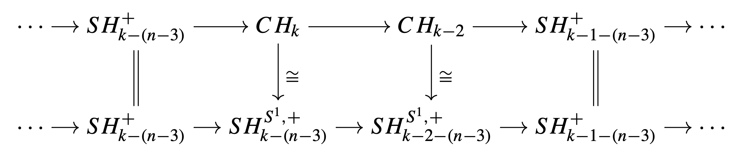
where we removed all decorations \( (W, \omega) \) for brevity.
As a consequence of this result, one sees that the positive part of \( S^1 \)-equivariant symplectic homology can be used as a substitute for linearized contact homology, even when the latter is not well defined owing to transversality issues for moduli spaces of holomorphic curves. It is indeed possible in a number of situations to find generic almost complex structures and Hamiltonian functions to make the moduli spaces for symplectic homology regular, because these geometric structures are time-dependent, unlike in contact homology. In situations where some Reeb vector field for \( (M, \xi) \) does not have any contractible orbit, it is possible to define \( SH^{S^1, +}(M, \xi) \) using the symplectization instead of a symplectic filling. This invariant has mostly been used when \( (W, \omega) \) is a Liouville manifold. In this spirit, Gutt and Hutchings [e59] used this invariant to construct a sequence of symplectic capacities for star-shaped domains in \( \mathbb{R}^{2n} \), leading to new applications to some symplectic embedding problems.
Using this relation between linearized contact homology and the positive part of \( S^1 \)-equivariant symplectic homology, it is possible to revisit Theorem 3.1 and to give an alternative proof via symplectic geometry. The key point is that symplectic homology, as well as its \( S^1 \)-equivariant counterpart, both vanish in the case of a subcritical Stein manifold. This is due to the fact that these manifolds factor as the product of a Stein manifold with \( \mathbb{C} \), as shown by Cieliebak [e10]; see also Section 14.4 of [9]. The symplectic topology of Stein manifolds is also the subject of another chapter of this volume [e74]. The conclusion for symplectic homology then follows from the Künneth formula proved by Oancea [e23] and the fact that symplectic homology of \( \mathbb{C} \) vanishes. The Gysin exact sequence between symplectic homology and its \( S^1 \)-equivariant version then shows that the latter has the same rank in any degree of a given parity. But an easy inspection shows that the generators of its chain complex have nonnegative grading, so that \( S^1 \)-equivariant symplectic homology vanishes as well. Once this is established, the tautological exact sequence \eqref{eq:SHtauto} in the \( S^1 \)-equivariant case shows that the positive part of \( S^1 \)-equivariant symplectic homology (or in other words linearized contact homology) is isomorphic to \( H^{S^1}_*(W) \). Since the circle acts on the \( \theta \in S^1 \) variable of the Hamiltonian and not on \( W \), the latter homology is isomorphic to \( H_*(W) \otimes H_*(BS^1) \), and this coincides with the result given in Theorem 3.1.
3.5. Variants of contact homology
Embedded Contact Homology (ECH) was introduced by Hutchings; for an introduction see, for example, [e41]. This theory also consists in a chain complex whose differential counts holomorphic curves in a symplectization, but as suggested by the name ECH, only embedded holomorphic curves are considered. It is also a four-dimensional theory, because embedding control is made possible by positivity of intersection, which is a four-dimensional phenomenon. Another major difference between ECH and contact homology is that the former turns out to be a topological invariant of the 3-manifold under consideration, and does not depend on the contact structure which is used to define it, because it is isomorphic to the Seiberg–Witten Floer cohomology defined by Kronheimer and Mrowka [e25]. This isomorphism was established by Taubes, who used it to prove [e24] the Weinstein conjecture in dimension three. This very important conjecture will be discussed in more details in Section 4.4. ECH is also a formidable tool to study symplectic embedding problems and to obtain sharp restrictions on them via the so-called ECH capacities. All this is well outside our present scope and certainly deserves its own volume.
Sutured contact homology was introduced by Colin, Ghiggini, Honda and Hutchings [e33]. It is a generalization of contact homology which is defined for a certain class of contact manifolds with boundary, called sutured contact manifolds. The latter are the contact analogue of symplectic manifolds with contact type boundary. Given a contact manifold \( (M, \xi) \) with boundary, one requires that the \( \partial M \) be transverse to a vector field preserving \( \xi \). Then, one restricts to contact forms \( \alpha \) for \( \xi \) so that the tangency locus of the Reeb field \( R_\alpha \) to \( \partial M \) is a smooth submanifold \( \Gamma \) on which \( \alpha \) restricts to a contact form: it is the suture of \( (M, \xi) \). Its complement \( \partial M \setminus \Gamma \) consists of regions \( R_\pm \) where \( \pm R_\alpha \) points outside \( M \), and \( (R_\pm, \alpha) \) are Liouville manifolds with convex boundary \( \Gamma \). Finally, the Reeb field \( R_\alpha \) is required, along the suture \( \Gamma \), to point from \( R_- \) to \( R_+ \) ; this condition corresponds to a convexity condition for the contact form \( \alpha \) along \( \partial M \). One can then complete such a contact manifold \( (M, \alpha) \) so that all closed Reeb orbits lie in the original manifold and all holomorphic curves in the corresponding symplectization that are asymptotic to these Reeb orbits do not leave a compact subset of the completed manifold. Sutured contact homology can then be defined in a similar way to contact homology. Golovko [e45] computed the sutured contact homology for universally tight contact structures on solid tori. This variant of contact homology can also lead to Legendrian invariants by considering the sutured contact homology of the complement of Legendrian submanifolds.
Local contact homology was introduced by Hryniewicz and Macarini [e46]. This is a homological invariant associated to a single closed Reeb orbit \( \gamma \), which is possibly degenerate. Intuitively, it measures the local contribution of this closed Reeb orbit to cylindrical or linearized contact homology of the whole contact manifold, after a perturbation of the contact form in order to replace \( \gamma \) with a collection of nearby nondegenerate closed Reeb orbits. It turns out that the rank of this invariant is bounded in any given grading and for any iteration of the orbit \( \gamma \). Applications of this invariant include a generalization of Gromoll–Meyer’s theorem on the existence of infinitely many simple periodic orbits, resonance relations and conditions for the existence of nonhyperbolic periodic orbits.
Momin [e34] defined a version of cylindrical contact homology for orbit complements in dimension three. More precisely, given a link \( L \) in a contact 3-manifold \( (M, \xi) \), we restrict ourselves to contact forms \( \alpha \) such that \( L \) is realized by a collection of closed Reeb orbits. We define a graded module that is linearly generated by closed Reeb orbits \( \gamma \) of such contact forms in \( M \setminus L \), such that \( \gamma \) realizes a fixed free homotopy class \( [a] \) in this manifold. It is equipped with differential counting rigid holomorphic cylinders that are contained in the symplectization of \( M \setminus L \). Under suitable assumptions on \( L \), \( \alpha \) and \( [a] \), this is a chain complex whose homology has some invariance properties. This invariant can be used to establish some implied existence results: assuming that the Reeb flow admits some closed orbits with certain properties, one deduces that it has a certain number of other closed orbits in some free homotopy class.
The Euler characteristic is a convenient numerical invariant for chain complexes of finite rank. When the chain complex for linearized or cylindrical contact homology has finite rank in any given degree, but has a total rank which is infinite, it is sometimes possible to define its mean Euler characteristic. In the case of cylindrical contact homology, this was defined by van Koert [e18] as \[ \chi(M,\xi) = \lim_{N \to \infty} \frac1N \sum_{m = -N}^N (-1)^m \textrm{rank } CH^\mathrm{ cyl}_m(M,\xi). \] A huge advantage of this invariant is that it can be computed in terms of closed Reeb orbits and their Conley–Zehnder indices, without having to compute the contact homology differential, or, in other words, having to find all rigid holomorphic curves. Going beyond distinguishing contact manifolds, in [e36] Frauenfelder, Schlenk and van Koert used this invariant to study some contact embedding problems. This work was then used by Kang [e40] to prove the existence of at least two closed Reeb orbits on some classes of contact manifolds (see Section 4.4 below for more advanced results in this direction). The mean Euler characteristic was also used by Chiang, Ding and van Koert [e43] to prove that some fibered Dehn twists are not symplectically isotopic to the identity relative to the boundary. Espina [e44] extended this notion to a broader class of contact manifolds; she also studied the effect of subcritical contact surgery on this invariant.
4. Applications of contact homology
4.1. Distinguishing contact structures
Since contact homology and its variants are invariants of contact manifolds, their first applications consist in distinguishing contact structures on a given closed manifold \( M \). The first application of this nature was obtained by Ustilovsky as the main result of his PhD thesis under Eliashberg’s supervision [e8], with \( M = S^{4k+1} \) for any integer \( k \ge 1 \). The Brieskorn manifolds, defined as the transverse intersection of the singular complex hypersurface \( z_0^{a_0} + z_1^{a_1} + \dots + z_n^{a_n} = 0 \) with a small unit sphere around the origin, are diffeomorphic to \( S^{4k+1} \) when \( n = 2k+1 \), \( a_1 = \dots = a_{2k+1} = 2 \) and \( 2 < a_0 = p \equiv \pm 1 \mod 8 \). The 1-forms \begin{equation} \label{eq:brieskorn} \alpha_{(a_0, \dots, a_n)} = \frac{i}8 \sum_{j=0}^n a_j (z_j d{\bar z}_j - {\bar z}_j dz_j)\tag{4.1} \end{equation} are contact forms and we denote by \( \xi_p \) the corresponding contact structures on \( S^{4k+1} \) in the above particular case.
Note that contact structures can sometimes be distinguished by their classical invariants, defined using tools from algebraic topology. These are all determined by the formal homotopy class of the contact structure, which is defined as its homotopy class as a complex vector subbundle of the tangent bundle of the ambient manifold. For spheres of dimension \( 4k+3 \) with \( k \ge 1 \), there are infinitely many formal homotopy classes, and one can show that the contact structures obtained as above fall into distinct classes, so contact homology is not needed to distinguish those contact structures. On the other hand, for spheres of dimension \( 4k+1 \) with \( k \ge 1 \), there are only finitely many such formal homotopy classes, so the above construction leads to infinitely many contact structures having the same formal homotopy classes. In this case, it is very useful to compute their cylindrical contact homology.
This explicit calculation was possible thanks to the fact that the Conley–Zehnder indices of all closed Reeb orbits of \( \alpha_p \), which is a suitable perturbation of the 1-form \( \alpha_{(a_0, \dots, a_n)} \) in Equation \eqref{eq:brieskorn}, have the same parity, so that \( \partial^\mathrm{ cyl} = 0 \). The result of this calculation shows in particular that cylindrical contact homology remembers the value of \( p \), and the invariance of contact homology then implies that \( S^{4k+1} \) admits infinitely many pairwise nondiffeomorphic contact structures.
At the time Ustilovsky’s paper [e7] appeared, invariance of cylindrical contact homology in the presence of contractible closed Reeb orbits was not fully established, due to the possible presence of multiply covered holomorphic planes with a positive asymptote at such orbits, for which transversality cannot be achieved with a generic almost complex structure. Using the considerations explained in Section 3.4, Gutt [e56] gave a complete proof of the existence of infinitely many pairwise nondiffeomorphic contact structures on \( S^{4k+1} \) using the positive part of \( S^1 \)-equivariant symplectic homology as a well-established substitute for cylindrical contact homology in Theorem 4.1.
Using the same techniques, Fauck [e64] extended this result to all contact manifolds \( (M, \xi) \) of dimension \( 4k+1 \) admitting an exact symplectic filling such that noncontractible loops in \( M \) are not contractible in the filling either, and satisfying an additional assumption (asymptotically finitely generated) on the quantity of closed Reeb orbits with a given Conley–Zehnder index.
In dimension three, one can construct infinitely many nondiffeomorphic contact structures on a toroidal manifold \( M \) by cutting this manifold
along an incompressible torus and inserting a domain of the form \( T^2 \times [0, 2k\pi] \) for some integer \( k \ge 1 \) equipped with the contact structure
\( \xi_k = \ker (\cos(\theta) \,dx + \sin(\theta) \,dy) \), where \( x \) and \( y \) are global angular coordinates on \( T^2 \) and \( \theta \in [0, 2k\pi] \). These contact
structures can then be distinguished by their Giroux torsion, which is defined as the largest integer \( k \) such that the above contact domain
can be embedded in a given contact manifold. As this invariant is difficult to compute, it is simpler to use cylindrical contact homology, and this
was done
in
[e19]
by Colin and the present author.
In dimensions greater than three,
Massot,
Niederkrüger
and
Wendl
[e37]
generalized this construction
by producing contact structures \( \xi_k \) on \( T^2 \times M \) for any integer \( k \ge 1 \), where \( M \) are suitable contact manifolds of arbitrary dimensions,
equipped with
two contact forms \( \alpha_+ \) and \( \alpha_- \), in such a way that
\[
\xi_k = \ker \biggl(\frac{1+ \cos kx}2 \alpha_+ + \frac{1-\cos kx}2 \alpha_-
+ \sin kx \, dy\biggr).
\]
As in dimension three, these contact structures are distinguished using cylindrical contact homology.
In order to compute the contact homology or one of its variants, it is useful to take advantage of the symmetries of natural contact forms and their associated Reeb vector fields. For instance, the Reeb flow associated to the contact form \( \alpha_{(a_0, \dots, a_n)} \) in Equation \eqref{eq:brieskorn} is periodic, though all simple closed Reeb orbits do not have the same period. In other words, the quotient of \( S^{4k+1} \) by the Reeb flow is a symplectic orbifold. In more general situations, one could have submanifolds of \( (M,\xi) \) that are foliated by closed Reeb orbits of different periods. Such contact forms are degenerate, but one can impose the condition that the eigenspace of the eigenvalue 1 coincide with the tangent space of these foliated submanifolds, in order to retain a nondegeneracy property in the transverse directions. This is analogous to the notion of a Morse–Bott function. It is possible to compute contact homology using such a contact form [e13]. To summarize, the generators of the Morse–Bott complex for contact homology are critical points of auxiliary Morse functions chosen on the foliated submanifolds. The differential counts cascades, which consist of an alternance between fragments of gradient trajectories for the auxiliary Morse functions and \( J \)-holomorphic curves for an almost complex structure \( J \) which is compatible with the Morse–Bott geometric data. The fragments joining two holomorphic curves can have an arbitrary finite length, while those reaching the generators of the complex are parametrized by a half-line. For more details, see, for example, [e28].
In particular, the calculation of cylindrical contact homology in Theorem 4.1 can be made using the contact form \( \alpha_{(a_0, \dots, a_n)} \) in Equation \eqref{eq:brieskorn} without any perturbation. The corresponding Reeb flow is given by \( \varphi^{R_\alpha}_t(z_0, \dots, z_n) = (e^{4it/p} z_0, e^{2it} z_1, \dots, e^{2it} z_n) \), so that orbits with \( z_0 =0 \) have minimal period \( \pi \) while orbits with \( z_0\neq 0 \) have minimal period \( p\pi \). It turns out that the space of closed Reeb orbits with period \( kp\pi \) is homeomorphic to \( \mathbb{C}\mathrm{P}^{n-1} \) for all \( k \ge 1 \), while the space of closed Reeb orbits with period \( k \pi \) has the same singular homology as \( \mathbb{C}\mathrm{P}^{n-2} \) for all \( k \ge 1 \) not multiple of \( p \). Due to the \( S^1 \)-symmetry induced by the Reeb flow, there are no rigid holomorphic curves, so that cylindrical contact homology will be a repetition of the singular homology of the orbit spaces for periods \( (kp+1)\pi, \dots (kp+p-1)\pi, (k+1)p\pi \) for \( k \ge 0 \), with suitable grading shifts due to the Conley–Zehnder index. It follows easily that there is a repetitive pattern with respect to the grading for the dimensions of cylindrical contact homology, a fact which is not completely obvious from the statement of Theorem 4.1.
More generally, van Koert [e26] computed the cylindrical contact homology for Brieskorn manifolds with many different values of the exponents \( a_0, \dots, a_n \). As a consequence of this, he exhibited large classes of contact manifolds admitting infinitely many nondiffeomorphic contact structures. More results on this class of contact manifolds were surveyed by Kwon and van Koert [e48], using \( S^1 \)-equivariant symplectic homology. Similar computations were used by Boyer, Macarini and van Koert [e51] to study the space of positive Sasakian structures on these manifolds.
Other applications of the above Morse–Bott techniques were obtained by Abreu and Macarini [e35] who computed the cylindrical contact homology combinatorially for large classes of toric contact manifolds. In particular they exhibited infinitely many nondiffeomorphic contact structures on \( S^2 \times S^3 \) with vanishing first Chern class. In a similar spirit, Boyer and Pati [e42] established criteria for contact structures on \( S^3 \)-bundles over \( S^2 \) to be nondiffeomorphic, even when they are not distinguished by their first Chern class. Returning to toric contact manifolds, Marinkovi&cacute [e58] related the cylindrical contact homologies of two such manifolds, when one is obtained from the other by a contact blow-up.
4.2. Topology of the space of contact structures
In view of Gray’s stability theorem, distinguishing contact structures amounts to the study of the set of connected components of the space of contact structures, modulo the contact mapping class group. It turns out that contact homology can also be used to study higher homotopy groups of the space of contact structures. Given an odd dimensional manifold \( M \), Let us denote by \( \Xi(M) \) the set of all contact structures on \( M \), equipped with the topology induced by the Grassmannian manifold of all codimension one subbundles of the tangent bundle \( TM \). Given a contact structure \( \xi_0 \) on \( M \), one can think of elements in \( \Pi_k(\Xi(M), \xi_0) \) as homotopy classes of families \( \xi_{(t_1, \dots, t_k)} \) of contact structures on \( M \) parametrized by \( [0,1]^k \), and which coincide with \( \xi_0 \) if \( t_j = 0 \) or 1 for some \( j \in \{ 1, \dots, k \} \). Given such a \( k \)-parameter family, one can construct a \( k-1 \)-parameter family of symplectic cobordisms \( (\mathbb{R} \times M, \omega_{(t_2, \dots, t_k)}) \), all interpolating from \( (M, \xi_0) \) to itself, and which coincide with the symplectization of \( (M, \xi_0) \) if \( t_j = 0 \) or 1 for some \( j \in \{ 2, \dots, k \} \). To carry out this construction, pick a family of contact forms \( \alpha_{(t_1, \dots, t_k)} \) for \( \xi_{(t_1, \dots, t_k)} \) which coincides with a fixed contact form \( \alpha_0 \) for \( \xi_0 \) when \( t_j = 0 \) or 1 for some \( j \in \{ 1, \dots, k \} \). Choose a smooth decreasing function \( f : \mathbb{R} \to [0,1] \) such that \( f(t) = 0 \) if \( t \) is sufficiently large, \( f(t) = 1 \) if \( t \) is sufficiently small and \( f \) varies very slowly. Then \( \omega_{(t_2, \dots, t_k)} = d(e^t \alpha_{(f(t), t_2, \dots, t_k)}) \) is the desired family of symplectic forms.
Counting rigid holomorphic curves in this family of symplectic cobordisms leads to maps descending to homotopy groups of \( \Xi(M) \). More precisely, one obtains group morphisms [e22] \[ \eta_1 : \pi_1(\Xi(M), \xi_0) \to \textrm{Aut}(CH^\mathrm{ cyl}(M, \xi_0)) \] and \[ \eta_k : \pi_k(\Xi(M), \xi_0) \to \textrm{End}_{1-k}(CH^\mathrm{ cyl}(M, \xi_0)) \] for \( k \ge 2 \), where for a graded module \( V \), \( \textrm{Aut}(V) \) denotes the nonabelian group of degree 0 automorphisms of \( V \) and \( \textrm{End}_{1-k}(V) \) denotes the additive group of degree \( 1-k \) endomorphisms of \( V \). These morphisms can be used to detect nontrivial elements in the homotopy groups of \( \Xi(M) \). For example, \( \pi_1(\Xi(T^3), \xi_0) \) contains an infinite cyclic subgroup for any tight contact structure \( \xi_0 \). This subgroup is generated by loops \( t \in \mathbb{R}/2\pi\mathbb{Z} \mapsto \ker(\cos(nz-t) \,dx + \sin(nz-t) \,dy) \in \Xi(T^3) \), where \( (x,y,z) \) are angular coordinates on \( T^3 \) and \( n \) is a positive integer. A similar statement holds for \( T^2 \)-bundles of \( S^1 \) and for \( T^5 \), using appropriate base points \( \xi_0 \). For a compact, orientable \( 2n \)-manifold \( Q \), \( \,\pi_{2n-1}(\Xi(ST^*Q), \xi_0) \) also contains an infinite cyclic subgroup, when \( \xi_0 \) is the canonical contact structure on the unit cotangent bundle \( ST^*Q \).
4.3. Tight vs. overtwisted
In the case of three-dimensional contact manifolds \( (M^3, \xi) \), Eliashberg introduced the notion of overtwisted contact structures: a contact structure \( \xi \) is said to be overtwisted if there exists a smooth embedding of the 2-disk in \( M^3 \) such that, along the boundary of this disk, its tangent space coincides with \( \xi \); in that case, this embedded 2-disk is called an overtwisted disk. If no such disk exists in \( (M, \xi) \), then \( \xi \) is said to be tight. This dichotomy between tight and overtwisted contact structures is of special importance because Eliashberg proved [1] that overtwisted contact structures satisfy an h-principle and are therefore classified in purely topological terms. In contrast, tight contact structures tend to have a geometric interest: for example, they include, but are not limited to, those contact structures that are induced by a symplectic filling. Since the existence of overtwisted contact structures is a purely topological phenomenon, it makes sense that contact homology has nothing to say about them. The following result was proved in [e21] by Yau, while a different proof of the same was given in the appendix by Eliashberg.
In dimension greater than three, there was no notion of overtwisted contact structures at the time of the above result. However, some classes of contact manifolds in arbitrary dimensions were singled out as sharing some geometric properties with overtwisted contact manifolds, and contact homology was proved to vanish for some of these classes. This includes the class of contact structures obtained by a negative stabilization of an open book decomposition supporting another contact structure [e32]. Another significant class consisted of the so-called PS-overtwisted contact structures [e20], defined using a higher dimensional generalization of the overtwisted disk. An unpublished result (see Theorem 4.10 of [e28]) showed that contact homology vanishes for such contact manifolds as well. Moreover, the vanishing of contact homology was shown to be equivalent to the vanishing of the rational SFT or of the full SFT [e31].
This situation changed drastically when Borman, Eliashberg and Murphy [10] defined the notion of overtwisted contact structure in arbitrary dimension and established an h-principle for this class of contact structures. This celebrated result is the subject of another chapter in this volume [e75]. Let us simply mention here that subsequent results by Casals, Murphy and Presas [e60] implied that contact homology vanishes for overtwisted contact manifolds of arbitrary dimensions, and this superseded all of the above-mentioned vanishing results.
In view of these vanishing results, it is natural to ask whether contact homology detects overtwisted contact structures; in other words, does \( CH(M, \xi) = 0 \) imply that \( \xi \) is overtwisted? This important question was answered negatively by Avdek [e70]. More precisely, he showed that contact \( +1 \)-surgery on the standard contact 3-sphere along a Legendrian link having a component which is a right-handed trefoil produces contact manifolds with vanishing contact homology. One of these contact manifolds was already known to be tight, based on arguments from Heegaard Floer homology.
As a consequence of the above groundbreaking result by Borman, Eliashberg and Murphy, it became interesting to construct and study tight contact manifolds in dimension greater than three. In particular, a former construction [e11] of a contact structure on \( T^2 \times M \) based on an open book decomposition supporting a contact structure on \( M \) was studied in this new light by several groups of researchers. Bowden, Gironella, Moreno and Zhou [e71] used contact homology to show that some of these contact manifolds are tight. This, in turn, allowed them to construct many examples of tight contact manifolds without symplectic fillings. More recently, Avdek and Zhou [e72] showed that all contact structures obtained from the above construction are tight, by computing the contact homology of a suitable covering of \( T^2 \times M \).
4.4. Dynamical complexity
Reeb vector fields constitute a remarkable class of nonvanishing vector fields, and their study from a dynamical point of view is of great interest. In particular, they generalize the geodesic flow in the case of unit cotangent bundles equipped with their canonical contact structures. A central question about the dynamical properties of Reeb vector fields is the celebrated Weinstein conjecture, which states in its modern form that any Reeb vector field on a closed contact manifold admits a periodic orbit. This conjecture motivated a lot of intensive work in contact geometry, leading to a plethora of interesting results. Indeed, contact homology can be thought of as an especially appropriate tool to prove this conjecture for a given closed contact manifold \( (M, \xi) \). It suffices to show that \( CH(M,\xi) \neq \mathcal{R} \), or that \( CH^\mathrm{ cyl}(M, \xi) \neq 0 \), or that \( CH^\varepsilon(M,\xi) \neq 0 \) for some augmentation \( \varepsilon \), to deduce that the Weinstein conjecture holds for \( (M,\xi) \). Hofer’s proof [e2] of the Weinstein conjecture for overtwisted contact 3-manifolds can be reinterpreted as the main step of the proof outlined in Section 4.3 that contact homology vanishes for such manifolds. All computations of contact homology and its variants made so far establish the Weinstein conjecture for the corresponding contact manifolds. However, the case of general closed contact manifolds still eludes us, and in comparison with ECH it seems that we are still lacking a general structural result for contact homology in order to prove the Weinstein conjecture in dimensions greater than three.
Instead of looking for a single closed Reeb orbit in very general contact manifolds, one can turn to a more quantitative version of the Weinstein conjecture for some specific classes of contact manifolds. The goal here is to establish some (possibly sharp) lower bound for the number of geometrically distinct closed Reeb orbits on a given contact manifold. Contact homology is a useful tool in that respect, but its rank does not directly provide the desired lower bound, as multiple covers of a given closed orbit are considered as separate generators of the contact chain complex, but are not geometrically distinct from the underlying simple closed Reeb orbit. In order to extract information about those simple orbits, it is necessary to understand thoroughly how the Conley–Zehnder index behaves for iterated orbits. The necessary information is contained in the so-called common index jump theorem, due to Long and Zhu ([e12], Theorem 4.3). Combining cylindrical contact homology with this result, Abreu and Macarini [e57], Gutt and Kang [e53], and Ginzburg and Gürel [e63] (using more symplectic techniques), proved independently that a star-shaped hypersurface in \( \mathbb{R}^{2n} \), equipped with the restriction of the standard contact form, has at least \( n \) simple closed Reeb orbits, under the assumption that the contact form is nondegenerate and dynamically convex. This last assumption means that all closed Reeb orbits have Conley–Zehnder index at least \( n+1 \). Similar results hold for prequantization bundles [e57], with as lower bound the sum of the Betti numbers of the base, under some assumptions of a similar nature.
Another approach to the abundance of closed Reeb orbits is to consider the number \( N_T(\alpha) \) of closed Reeb orbits with period at most \( T \) corresponding to the contact form \( \alpha \), and to study the growth rate of \( N_T(\alpha) \) as \( T \) tends to infinity. Since the period of a closed Reeb orbit coincides with its action, which decreases under the differential, the module generated by \( \mathcal{P}^{\le T}_\alpha \) forms a subcomplex for contact homology, and the rank of its homology \( CH^{\mathrm{cyl}}_{\le T}(M, \alpha) \) provides a lower bound for \( N_T(\alpha) \). Vaugon [e47] showed that this growth rate is independent of the choice of a contact form for a given contact structure. She also showed that this growth rate is exponential in the case of a closed 3-manifold such that its JSJ decomposition contains a hyperbolic component that fibers over the circle. This was motivated by work of Colin and Honda [e38], in which they computed the cylindrical or linearized contact homology for contact 3-manifolds supported by an open book decomposition with special types of monodromies, including periodic or pseudo-Anosov maps. They also showed that linearized contact homology has exponential growth for some pseudo-Anosov monodromies.
The complexity of the flow \( \varphi \) of a vector field, seen as a dynamical system, can be measured by its topological entropy \( h_{\mathrm{top}}(\varphi) \). It is especially important to be able to distinguish between dynamical systems having vanishing versus positive topological entropy. Using cylindrical contact homology, Alves [e54] established a positive lower bound for the topological entropy of the Reeb flow in the case of the same class of closed 3-manifolds as above, as well as for contact 3-manifolds obtained by a Foulon–Hasselblatt surgery on the unit cotangent bundle of a closed surface along the Legendrian lift of a separating geodesic. He also proved a similar result for closed contact 3-manifolds admitting a Reeb flow which is Anosov [e52]. Note that other results of the same nature but for other classes of contact manifolds can be obtained using a variant of Legendrian contact homology, but the latter tool is outside our present scope. In the same period, Foulon, Hasselblatt and Vaugon [e66] improved the above results to the case of contact 3-manifolds obtained by a Foulon–Hasselblatt surgery on the unit cotangent bundle of a closed surface along the Legendrian lift of any closed geodesic.
4.5. Other applications
Let us finally mention some other applications of contact homology that we will not develop in detail in this text.
The celebrated Gromov nonsqueezing theorem is one of the cornerstones of symplectic topology. Eliashberg, Kim and Polterovich [6] used contact homology to establish a contact geometric version of this theorem, with a crucial distinction between large-scale and small-scale phenomena. They also discover a relation to the existence of a partial order on the universal covering of the contactomorphism group of the contact manifold under consideration. This initiated a whole new avenue of research, which we do not develop further, as it is the subject of another chapter of this volume [e78].
As we saw in Section 3.4, symplectic homology and its \( S^1 \)-equivariant counterpart both vanish in the case of subcritical Stein manifolds. This also means that the attachment of a subcritical handle to a symplectic manifold with convex boundary does not change these invariants, and that its effect on linearized contact homology is purely topological. However, the situation drastically changes when attaching a critical handle along a Legendrian sphere \( \Lambda \) in the contact boundary. Together with the present author, Ekholm and Eliashberg described the effect of such an operation on the above invariants using long exact sequences involving suitable variants of the Legendrian contact homology of \( \Lambda \) [8]. This first result has many ramifications and applications, which we do not detail here, as it is the subject of another chapter of this volume [e73].
