by Terence Tao
Cast a stone into a still lake. There is a large splash, and waves begin radiating out from the splash point on the surface of the water. But, as time passes, the amplitude of the waves decays to zero.
This type of behavior is common in physical waves, and also in the partial differential equations used in mathematics to model these waves. Let us begin with the classical wave equation \begin{equation} \label{one} -\partial_{tt} u + \Delta u = 0, \end{equation}
where \( u \colon \mathbb{R} \times \mathbb{R}^3 \rightarrow \mathbb{R} \) is a function of both time \( t \in \mathbb{R} \) and space \( x \in \mathbb{R}^3 \), which is a simple model for the amplitude of a wave propagating at unit speed in three-dimensional space; here \begin{equation*} \Delta = \frac{\partial^2}{\partial x^2_1} + \frac{\partial^2}{\partial x^2_2} + \frac{\partial^2}{\partial x^2_3} \end{equation*}
denotes the spatial Laplacian. One can verify that one has the family of explicit solutions \begin{equation} u(t, x) = \frac{F(t + |x|) - F(t - |x|)}{|x|} \end{equation}
to \eqref{one} for any smooth, compactly supported function \( F \colon \mathbb{R} \rightarrow \mathbb{R} \), where \begin{equation*} |x| = \sqrt{x^2_1 + x^2_2 + x^2_3} \end{equation*}
denotes the Euclidean magnitude of a position \( x \in \mathbb{R}^3 \). The dispersive nature of this equation can be seen in the observation that the amplitude \begin{equation*} \sup_{x\in\mathbb{R}^3} |u(t, x)| \end{equation*}
of such solutions decays to zero as \( t \rightarrow \pm \infty \), whilst other quantities such as the energy \begin{equation*} \int_{\mathbb{R}^3} \frac{1}{2} |\partial_t u(t, x)|^2 + \frac{1}{2} |\nabla u(t, x)|^2\, dx \end{equation*}
stay constant in time (and in particular do not decay to zero).
The wave equation can be viewed as a special case of the more general linear Klein–Gordon equation \begin{equation} \label{three} -\partial_{tt} u + \Delta u = m^2 u, \end{equation}
where \( m \geq 0 \) is a constant. Even more important is the linear Schrödinger equation, which we will normalize here as \begin{equation} \label{four} i\partial_t u + \frac{1}{2} \Delta u = 0, \end{equation}
where the unknown field \( u \colon \mathbb{R} \times \mathbb{R}^3 \rightarrow \mathbb{C} \) is now complex-valued. There are also nonlinear variants of these equations, such as the nonlinear Klein–Gordon equation \begin{equation} \label{five} - \partial_{tt} u + \Delta u = m^2 u + \lambda |u|^{p-1} u, \end{equation}
and the nonlinear Schrödinger equation \begin{equation} \label{six} i\partial_t u + \frac{1}{2}\Delta u = \lambda |u|^{p-1} u, \end{equation}
where \( \lambda = \pm 1 \) and \( p > 1 \) are specified parameters. There are countless other further variations (both linear and nonlinear) of these dispersive equations, such as Einstein’s equations of general relativity, or the Korteweg–de Vries equations for shallow water waves.

An important way to capture dispersion mathematically is through the establishment of dispersive inequalities that assert, roughly speaking, that if a solution \( u \) to one of these equations is sufficiently localized in space at an initial time, \( t = 0 \), then it will decay as \( t \rightarrow\infty \). (If a solution \( u \) is not localized enough in space initially, it does not need to decay; consider for instance the traveling wave solution \begin{equation*} u(t, x) = F(t - x_1) \end{equation*}
to the wave equation \eqref{one}.) This decay has to be measured in suitable function space norms, such as the \( L^{\infty}_x (\mathbb{R}^3) \) norm.
One can represent any solution \( u \) to the linear Schrödinger equation explicitly in terms of the initial data \( u(0) \) by the formula \begin{equation*} u (t,x)=\frac{1}{(2\pi it)^{3/2}}\int_{\mathbb{R}^3} e^{-i|x-y|^2/2t} u (0,y)\,dy \end{equation*}
for all \( t \neq 0 \) and \( x \in \mathbb{R}^3 \), where the quantity \( (2\pi it)^{3/2} \) is defined using a suitable branch cut. From the triangle inequality, this immediately gives the dispersive inequality \begin{equation} \|u(t)\|_{L^{\infty}_x(\mathbb{R}^3 )} \leq \frac{1}{(2\pi |t|)^{3/2}}\|u(0)\|_{L_x^1(\mathbb{R}^3)}. \end{equation}
If the solution is initially spatially localized in the sense that the \( L^1 \) norm \begin{equation*} \|u(0)\|_{L^{1}_x(\mathbb{R}^3 )} \end{equation*}
is finite, then the solution \( u(t) \) decays uniformly to zero as \( t \rightarrow \pm \infty \). A similar (but slightly more complicated) dispersive inequality can also be obtained for solutions to the linear Klein–Gordon equation \eqref{three}.
On the other hand, solutions to the linear Schrödinger equation \eqref{four} satisfy the pointwise mass conservation law \begin{equation} \partial_t |u|^2 = \sum^3_{j=1} \partial_{x_j} \mathrm{Im} (\bar{u}\,\partial_{x_j} u). \end{equation}
From this, one can easily derive conservation of the spatial \( L^2 \) norm of the solution: \begin{equation*} \|u(t)\|_{L^2_x (\mathbb{R}^3)} = \|u(0)\|_{L^2_x (\mathbb{R}^3)} . \end{equation*}
In particular, the \( L^2 \) norm of the solution will stay constant in time, rather than decay to zero.
To reconcile this fact with the dispersive estimate, we observe that solutions to dispersive equations such as the linear Schrödinger equation spread out in space as time goes to infinity (much as the ripples on a pond do), allowing the \( L^{\infty} \) norm of such a solution to go to zero even while the \( L^2 \) norm stays bounded away from zero. As mentioned earlier, this effect can also be seen for the wave equation \eqref{one}.
The above analysis of the linear Schrödinger equation relied crucially on having an explicit fundamental solution at hand. What happens if one works with nonlinear (and not completely integrable) equations, such as \eqref{five} or \eqref{six}, in which no explicit and tractable formula for the solution is available? For linear equations (such as the wave or Schrödinger equation outside of an obstacle, or in the presence of potentials or magnetic fields) one can still hope to use methods from spectral theory to understand the long-time behavior (as is done for instance in the famous RAGE theorem of Ruelle (1969), Amrein–Georgescu (1973), and Enss (1977)). However, such methods are absent for nonlinear equations such as \eqref{five} or \eqref{six}, particularly when dealing with solutions that are too large for perturbative theory to be of much use.
Recall that in 1961, Morawetz proved the decay of solutions to the classical wave equation in the presence of a star-shaped obstacle. Morawetz used the “Friedrichs abc method,” in which one multiplied both sides of a PDE such as \eqref{five} or \eqref{six} by a multiplier \begin{equation*} a\,\partial_t u + b \cdot \nabla u + cu \end{equation*}
for well-chosen functions \( a \), \( b \), \( c \), integrated over a space-time domain, and rearranging using integration by parts and omitting some terms of definite sign, obtained a useful integral inequality. The key discovery of Morawetz (a version of which first appeared in work of Ludwig) was that this method was particularly fruitful when the multiplier was equal to the radial derivative \begin{equation*} \frac{x \cdot \nabla u}{|x|} \end{equation*}
of the solution (in some cases one also adds a lower-order term \( u/|x| \)).
In 1968, Morawetz applied this technique to study solutions \( u \) to the nonlinear Klein–Gordon equation \eqref{five}, assuming one is in the nonfocusing case with \( \lambda = m =+1 \). (In the focusing case \( \lambda = -1 \), the equation \eqref{five} admits “soliton” solutions that are stationary in time and thus do not disperse.) By using a multiplier of the above form, Morawetz obtained an inequality of the form \begin{equation} \label{nine} \int_{\mathbb{R}} \int_{\mathbb{R}^3} U(t, x)\, dx\, dt \leq C E(u(0)), \end{equation}
where \begin{equation*} U(t, x) =\frac{ |u(t, x)|^2 + |u(t, x)|^{p+1}}{|x|}. \end{equation*}
Here the constant \( C \) depends only on the exponent \( p \) and \( E(u(0)) \) is the energy: \begin{equation*} E(u(0)) = \int_{\mathbb{R}^3} \frac{1}{2} |\nabla u(0, x)|^2 + \frac{1}{2} |\partial_t u(0, x)|^2 +\frac{1}{p+1} |u(0, x)|^{p+1}\, dx. \end{equation*}
This type of estimate is now known as a Morawetz inequality. The key point here is that the left-hand side of the Morawetz inequality in \eqref{nine} contains an integration over the entire time domain \( \mathbb{R} \) (as opposed to a time integral over a bounded interval). It immediately rules out soliton-type solutions that move at bounded speed (as this would make the left-hand side of \eqref{nine} infinite). It forces some time-averaged decay of the solution near the spatial origin \( x = 0 \). For instance, it is immediate from \eqref{nine} that \begin{equation*} \frac{1}{T}\int_0^T \int_K |u(t, x)|^2\, dx\, dt \rightarrow 0 \end{equation*}
as \( T \rightarrow\infty \) for any compact spatial region \( K \subset \mathbb{R}^3 \).
Once one has some sort of decay estimate for a dispersive equation, it is often possible to “bootstrap” the estimate to obtain additional decay estimates. For instance one might use the decay estimate one already has to bound the right-hand side of a nonlinear PDE such as \eqref{five} or \eqref{six}, and then solve the associated (inhomogeneous) linear PDE to obtain a new decay estimate for the solution.
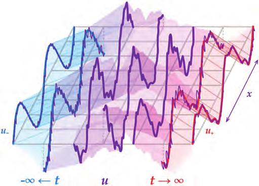
An early result of this type was developed by Morawetz and Strauss in 1975. They showed that for any finite energy solution \( u \) to the nonlinear Klein–Gordon equation \eqref{five} with \( \lambda = m = +1 \) and \( p = 3 \), the solution decays like a solution to the linear Klein–Gordon equation \eqref{three}. More precisely, there exist finite solutions \( u_+ , u_{-} \) to \eqref{three} such that \( u(t) - u_+ (t) \) (resp. \( u(t) - u_{-} (t) \)) goes to zero in the energy norm as \( t\rightarrow +\infty \) (resp. \( t \rightarrow -\infty \)). This can be developed further into a satisfactory scattering theory for such equations, which among other things gives a continuous scattering map from \( u_- \) to \( u_+ \) or vice versa. See Figure 2.
In the decades since Morawetz’s pioneering work, many additional Morawetz inequalities have been developed. For instance, in 1978, Lin and Strauss developed Morawetz inequalities for the nonlinear Schrödinger equation, and Morawetz herself discovered further such estimates for the wave equation outside of an obstacle. In more recent years, “interaction Morawetz inequalities” were introduced, which could control correlation quantities such as \begin{equation} \label{ten} \int_{\mathbb{R}} \int_{\mathbb{R}^3} \int_{\mathbb{R}^3} \frac{|u(t,x)|^2|u(t,y)|^p}{|x-y|}\,dx\,dy\,dt \end{equation}
for solutions \( u \) to the nonlinear Schrödinger equation \eqref{six}.
One way to view Morawetz inequalities is as an assertion of monotonicity of the radial momentum, which takes the form \begin{equation*} \int_{\mathbb{R}^3}(\partial_t u)\biggl(\frac{x}{|x|}\cdot \nabla u\biggr)\, dx \end{equation*}
for wave or Klein–Gordon equations, and \begin{equation*} \int_{\mathbb{R}^3}\operatorname{Im}\biggl(\bar{u}\frac{x}{|x|}\cdot \nabla u\biggr)\, dx \end{equation*}
for Schrödinger equations. Informally, this quantity is expected to be positive when waves propagate away from the origin, and negative when they propagate towards the origin. The intuition is that while waves can sometimes propagate towards the origin, eventually they will move past the origin and begin radiating away from the origin. However, in the absence of focusing mechanisms (such as a negative sign \( \lambda = -1 \) in the nonlinearity), the reverse phenomenon of outward net radial momentum being converted to inward net radial momentum cannot occur. Thus the radial momentum is always expected to be increasing in time.
On the other hand, under hypotheses such as finite energy, this radial momentum should be bounded. So by the fundamental theorem of calculus, the time derivative of the radial momentum should have a bounded integral in time. Intuitively, one expects this time derivative to be large when the solution has a strong presence near the origin, but not when the solution is far away from the origin. Far from the origin the radial vector field \begin{equation*} \frac{x}{|x|}\cdot \nabla \end{equation*}
behaves like a constant, and the radial momentum approaches a fixed coordinate of the total momentum. This explains why Morawetz inequalities tend to involve factors such as \( 1/|x| \) that localize the estimate to near the origin.
The Morawetz inequalities are indispensible as an ingredient in controlling the long-time behavior of solutions to a wide array of dispersive defocusing equations, including a number of energy-critical or mass-critical equations in which the analysis is particularly delicate and interesting; see for instance the texts [e1], [e3], [e4] for detailed coverage of these topics. They have also been successfully applied to many equations in general relativity (such as Einstein’s equations for gravitational fields), for instance to analyze the asymptotic behaviour around a black hole. The fundamental tools that Morawetz has introduced to the field of dispersive equations will certainly underlie future progress in this field for decades to come.
