Celebratio Mathematica

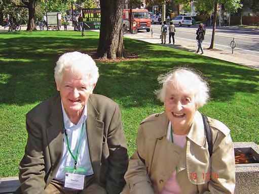
Cath­leen Mor­awetz was a force at the Cour­ant In­sti­tute when one of us (L.G.) ar­rived as a postdoc­tor­al fel­low. It was the last year of her dir­ect­or­ship, but she made the time to wel­come all new­comers. Her gen­er­os­ity of spir­it was un­matched — she en­cour­aged young people in every dis­cip­line, and her hu­mour and en­thu­si­asm were in­fec­tious.

When she began to study the de­cay prop­er­ties of acous­tic waves after impinging on an obstacle, es­sen­tially no gen­er­al res­ults were avail­able. To un­der­stand the rel­ev­ant is­sues, let us be­gin with the for­mu­la­tion of the prob­lem in terms of the gov­ern­ing lin­ear, scal­ar wave equa­tion in \( \mathbb{R}^3 \), with a for­cing term which is turned on for a fi­nite time: \begin{equation} \label{eleven} u_{tt} (\mathbf{x}, t) = \Delta u(\mathbf{x}, t) + f(\mathbf{x}, t). \end{equation} Here, \( \Delta u \) is the Lapla­cian op­er­at­or act­ing on the scal­ar func­tion \( u(\mathbf{x}, t) \) and \( f(\mathbf{x}, t) \) is nonzero only in the fi­nite time in­ter­val \( 0 \leq t \leq T \). We as­sume that we have zero ini­tial (Cauchy) data at time \( t = 0 \): \[ u(\mathbf{x}, 0) = 0\quad\text{ and } \quad u_t (\mathbf{x}, 0) = 0. \] We also as­sume that \( f(\mathbf{x}, t) \) is a smooth, com­pactly sup­por­ted and square in­teg­rable func­tion in space-time, such as \begin{equation} \label{twelve} f(\mathbf{x},t) = W(\|\mathbf{x} - \mathbf{x}_0\|)\, W\, \biggl(\frac{2t-T}{T}\biggr), \end{equation} where \( \mathbf{x}_0 \in \mathbb{R}^3 \) and \( W(x) \) is a stand­ard \( C^{\infty} \) bump func­tion such as \[ W(x) = \begin{cases} e^{-\frac{1}{1-x^2}} & \text{for } |x| < 1;\\ 0 & \text{otherwise}. \end{cases} \] Then, it is well known that \begin{equation} \label{thirteen} u(\mathbf{x}, t) = \frac{1}{4\pi}\int_{B_{\mathbf{x}_0} (1)} \frac{f (\mathbf{x}^{\prime}, t - \|\mathbf{x} - \mathbf{x}^{\prime}\|)}{\|\mathbf{x}-\mathbf{x}^{\prime}\|}\,d\mathbf{x}^{\prime}, \end{equation} where \( B_{\mathbf{x}_0} (1) \) de­notes the unit ball centered at \( \mathbf{x}_0 \). From this for­mula it is clear that at any point \( \mathbf{x} \) in space, the solu­tion first be­comes nonzero at \( t = d_{\min} \) , where \( d_{\min} \) is the dis­tance from \( \mathbf{x} \) to the closest point in \( B_{\mathbf{x}_0} (1) \). It van­ishes identic­ally at \( \mathbf{x} \) as soon as \( t > T + d_{\max} \), where \( d_{\max} \) is the dis­tance from \( \mathbf{x} \) to the farthest point \( B_{\mathbf{x}_0} (1) \).

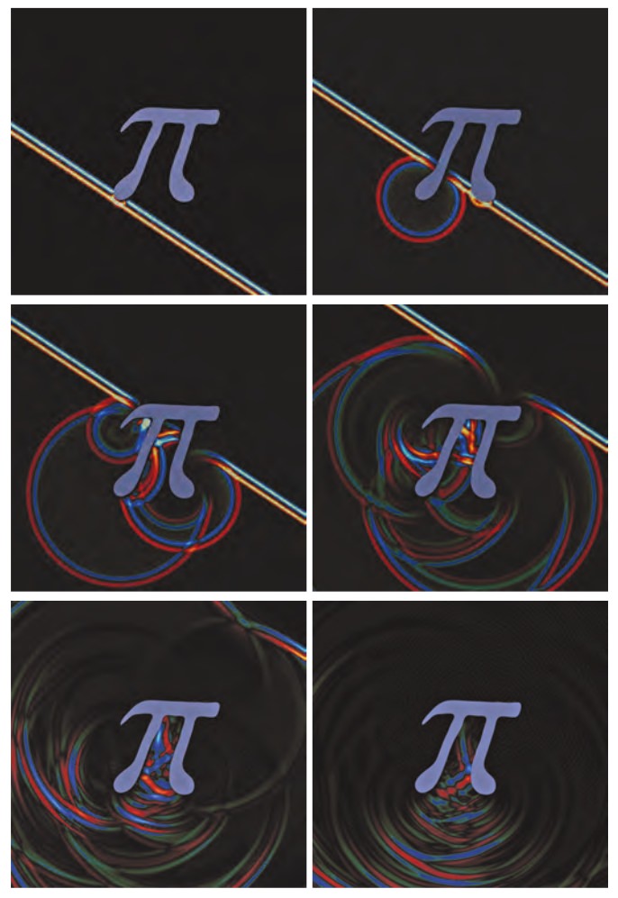
Sup­pose now that, rather than propagat­ing in free-space, the out­go­ing spher­ic­al wave­front em­an­at­ing from \( \mathbf{x}_0 \) hits an ob­ject as in Fig­ure 3. That is, we as­sume there is a “sound-soft,” smooth, bounded obstacle \( \Omega \) with bound­ary \( \partial\Omega \), which is at some dis­tance from \( B_{\mathbf{x}_0} (1) \), so that \[ \Omega \cap B_{\mathbf{x}_0} (1)= \emptyset .\] Then, us­ing the lan­guage of scat­ter­ing the­ory, the total acous­tic field is giv­en by \[ u(\mathbf{x}, t) + u^{\operatorname{scat}} (\mathbf{x}, t) ,\] where the scattered field sat­is­fies the ho­mo­gen­eous wave equa­tion \[ u^{\operatorname{scat}}_{tt} (\mathbf{x}, t) - \Delta u^{\operatorname{scat}} (\mathbf{x}, t) = 0 \] for \( t > 0 \), with ini­tial data \[ u^{\operatorname{scat}} (\mathbf{x}, 0) = 0 \] and \[ u^{\operatorname{scat}}_t (\mathbf{x}, 0) = 0 \] and Di­rich­let bound­ary con­di­tions \[ u^{\operatorname{scat}} (\mathbf{x}, t) = -u(\mathbf{x}, t) \] for \( x \in \partial\Omega \).

Let \( \mathbf{y} \) de­note some fixed point away from both the ball \( B_{\mathbf{x}_0} (1) \) and the obstacle \( \Omega \). The ques­tion is: can one prove that the scattered field de­cays at \( \mathbf{y} \), and if so, at what rate? Very little pro­gress had been made on this ques­tion un­til 1959, when Wil­cox pub­lished a short note show­ing that in the case of a spher­ic­al obstacle, an ex­act solu­tion could be ex­pressed in terms of spher­ic­al har­mon­ics. From this, Wil­cox was able to con­clude that the solu­tion de­cays ex­po­nen­tially fast. While an im­port­ant step, his res­ult yiel­ded no sug­ges­tion as to how to pro­ceed in the gen­er­al case.

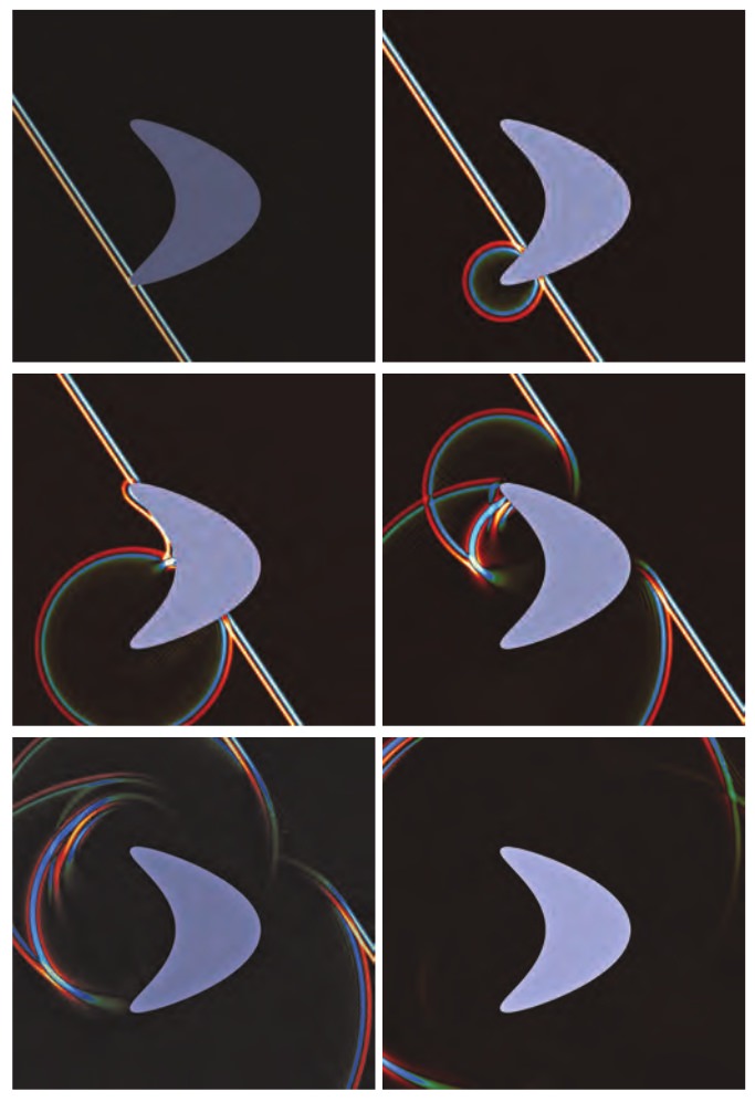
In 1961, Mor­awetz [1] made a crit­ic­al step for­ward. She showed that if the re­flect­ing obstacle is star-shaped, then the solu­tion to the wave equa­tion de­cays like \( t^{1/2} \). A re­gion \( \Omega \) is said to be star-shaped if there ex­ists a point \( \mathbf{p} \in \Omega \), such that for all \( \mathbf{x} \in \Omega \), the line seg­ment from \( \mathbf{p} \) to \( \mathbf{x} \) is con­tained in \( \Omega \). The ob­ject in Fig­ure 3, for ex­ample, is not star-shaped, while the ob­ject in Fig­ure 4 is. It is per­haps sur­pris­ing that for non-star-shaped obstacles, very little is un­der­stood to the present day.

The qual­it­at­ive dif­fer­ence in the be­ha­vi­or of waves re­flect­ing from obstacles that are not star-shaped and those that are is il­lus­trated in Fig­ures 3 and 4. In the first three pan­els of each fig­ure, as the in­com­ing wave hits the ob­ject, the scattered wave is clearly vis­ible, with en­ergy propagat­ing out­wards in all dir­ec­tions. In the next three pan­els, more of the en­ergy is car­ried away. In Fig­ure 3, some of the en­ergy re­mains be­hind for quite some time, and in the last pan­el a sig­ni­fic­ant amount of en­ergy has fo­cused in a small neigh­bor­hood. In Fig­ure 4, the en­ergy has propag­ated out­ward without sig­ni­fic­ant con­cen­tra­tion and ap­pears to de­cay much more rap­idly.

Mor­awetz’s writ­ing style was very much that of a storyteller. To get a sense of that, here is the be­gin­ning of the proof of the main the­or­em in her 1961 pa­per [1]:

The proof is based on en­ergy iden­tit­ies, i.e., quad­rat­ic in­teg­ral re­la­tions sat­is­fied by all solu­tions. This is one of the most power­ful tools for get­ting es­tim­ates for solu­tions of el­lipt­ic, hy­per­bol­ic or mixed equa­tions. The most fa­mil­i­ar iden­tity of this kind for the wave equa­tion is ob­tained by mul­tiply­ing \( u_{tt} = \Delta u \) by \( u_t \) and in­teg­rat­ing in the slab \( 0 \leq t \leq t_1 \); the res­ult­ing in­teg­ral iden­tity sat­is­fies the con­ser­va­tion of en­ergy. Here we use an­oth­er mul­ti­pli­er in the place of \( u_t \) in­tro­duced by Prot­ter for an­oth­er pur­pose. The sig­ni­fic­ance of us­ing al­tern­at­ive mul­ti­pli­ers has been fre­quently em­phas­ized by Friedrichs and is of­ten re­ferred to as Friedrichs’s \( a \), \( b \), \( c \)-meth­od. The mul­ti­pli­er here is \begin{equation} \label{fourteen} xu_x + yu_y + zu_z + tu_t + u \end{equation} and from the res­ult­ing iden­tity we con­clude that all the en­ergy is car­ried out­ward.

In truth, Mor­awetz was be­ing overly mod­est. It was her keen in­sight that al­lowed for the se­lec­tion of a mul­ti­pli­er which would yield the de­sired res­ult. The power and gen­er­al­ity of this ap­proach led to break­throughs in many wave propaga­tion prob­lems, with the state of the art col­lec­ted in Mor­awetz’s 1966 mono­graph “En­ergy iden­tit­ies for the wave equa­tion,” ori­gin­ally re­leased as a Cour­ant In­sti­tute tech­nic­al re­port.

A second ma­jor step for­ward in un­der­stand­ing the de­cay of waves scattered from star-shaped obstacles came in 1963, in joint work with Lax and Phil­lips. They showed that, in fact, such solu­tions de­cay ex­po­nen­tially (as they do for a sphere), not just as \( t^{-1/2} \). The proof re­lies on an ob­ser­va­tion of Lax and Phil­lips that there is a func­tion \( Z(t) \) which sat­is­fies the semig­roup prop­erty \begin{equation} \label{fifteen} Z(t + s) = Z(t)Z(s), \end{equation} and whose norm con­trols the de­cay of the solu­tion. In this con­text, Mor­awetz’s 1961 pa­per shows that for some time \( t = \tau \), \( |Z(\tau)| \) has de­cayed to less than one: \[ |Z(\tau)| < 1 = e^{-\alpha}\quad\text{ for some } \alpha > 0. \] That is enough to guar­an­tee ex­po­nen­tial de­cay! One simply writes \[ t = n\tau + t_1\quad\text{ where }t_1 < \tau, \] from which \[ |Z(t)| = |Z(t_1 )|\,|[Z(\tau)]^n | \leq |Z(t_1 )|e^{-\alpha n} = Ce^{-\alpha t/\tau}. \]

This situ­ation was stud­ied by Mor­awetz, Ral­ston, and Strauss in their 1977 art­icle, where they proved a re­mark­able ex­ten­sion of Mor­awetz’s earli­er res­ults; if the ob­ject \( \Omega \) does not trap rays, then the scattered wave de­cays ex­po­nen­tially. The proof in­volves the in­tro­duc­tion of an es­cape func­tion (a gen­er­al­iz­a­tion of the geo­met­ric in­tu­ition of an “es­cape path of fi­nite length”) and a dif­fer­ent mul­ti­pli­er from that in Mor­awetz’s 1961 pa­per. The use of such Mor­awetz mul­ti­pli­ers is now ubi­quit­ous in the ana­lys­is of PDEs.

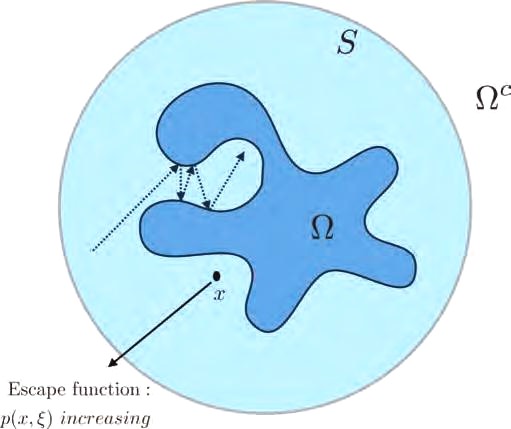
De­not­ing by \( S \) a sphere which con­tains the smooth scat­ter­er \( \Omega \), con­sid­er­ing \( \mathbf{x} \in S\backslash \Omega \), and let­ting \( \xi \) be a unit vec­tor in \( \mathbb{R}^3 \), \( p(\mathbf{x}, \xi) \) is said to be an es­cape func­tion if it is real-val­ued, \( C^{\infty} \), and, in­form­ally speak­ing, “strictly in­creas­ing along rays, \( \xi \) be­ing the ray dir­ec­tion at \( \mathbf{x} \).” Rays are said to be not trapped if the total path length in \( S\backslash \Omega \) is bounded and waves are said to be not trapped if the loc­al en­ergy in \( S\backslash \Omega \) de­cays to zero uni­formly. Without en­ter­ing in­to de­tails, Mor­awetz, Ral­ston, and Strauss showed (1) that if rays are not trapped, then there ex­ists an es­cape func­tion and (2) that if there ex­ists an es­cape func­tion, then waves are not trapped, from which the res­ult fol­lows.

In the study of lin­ear wave propaga­tion, much of our un­der­stand­ing comes from the fre­quency do­main — that is, ana­lyz­ing the Four­i­er trans­form of the wave equa­tion \eqref{eleven}: \begin{equation} \label{sixteen} - k^2 U(\mathbf{x}, k) - \Delta U(\mathbf{x}, k) = F(\mathbf{x}, k). \end{equation} De­pend­ing on the con­text, this is re­ferred to as the Helm­holtz or re­duced wave equa­tion. In 1968, Mor­awetz, to­geth­er with Don Lud­wig, began an in­vest­ig­a­tion of ex­ter­i­or scat­ter­ing from star-shaped sur­faces in the fre­quency do­main [2]. Two ma­jor res­ults were presen­ted there. First, they provided a key proof of the well-posed­ness of the scat­ter­ing prob­lem for sound-soft bound­ar­ies (ho­mo­gen­eous Di­rich­let bound­ary con­di­tions) with re­spect to the bound­ary data and for­cing term \( F(\mathbf{x}, k) \) in \eqref{sixteen}. They also in­tro­duced what are now called Mor­awetz iden­tit­ies for the Helm­holtz equa­tion. Second, they showed that the for­mu­las pro­duced by the the­ory of geo­met­ric­al op­tics are asymp­tot­ic to the ex­act solu­tion. The rel­ev­ant asymp­tot­ic re­gimes are il­lus­trated in Fig­ure 6.

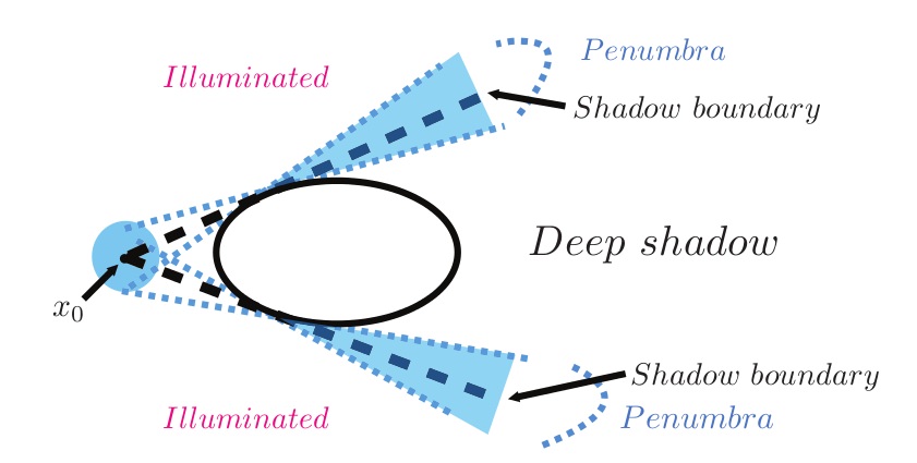
Without en­ter­ing in­to tech­nic­al de­tails, geo­met­ric­al op­tics is based on ex­pand­ing the in­com­ing and scattered waves in terms of a series in in­verse powers of the wavenum­ber \( k \) about the point \( \mathbf{x}_0 \) (see Fig­ure 6). Lud­wig had earli­er pro­posed an ex­pan­sion for the pen­um­bra re­gion as well. Mor­awetz and Lud­wig showed that all of these ex­pan­sions are truly asymp­tot­ic: to the solu­tion in the il­lu­min­ated re­gion and pen­um­bra, and asymp­tot­ic­ally zero in the deep shad­ow.

Al­though Mor­awetz her­self did little nu­mer­ic­al com­pu­ta­tion, her ana­lyt­ic work (es­pe­cially on mul­ti­pli­ers) has played a ma­jor role in the design of nu­mer­ic­al meth­ods. We can­not do justice to the lit­er­at­ure here, but refer the read­er to three re­cent pa­pers: one on ei­gen­value com­pu­ta­tion, one on fre­quency do­main scat­ter­ing, and one on time-do­main in­teg­ral equa­tions [e1] [e2] [e5]. We have only been able to scratch the sur­face of her leg­acy in this note. Her con­tri­bu­tions are pro­found and deep, and have changed the way we think about par­tial dif­fer­en­tial equa­tions. She was a won­der­ful friend and col­league and is greatly missed.